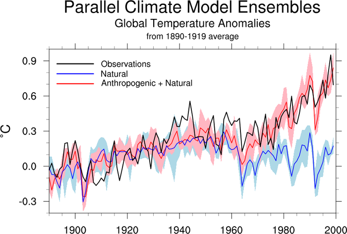
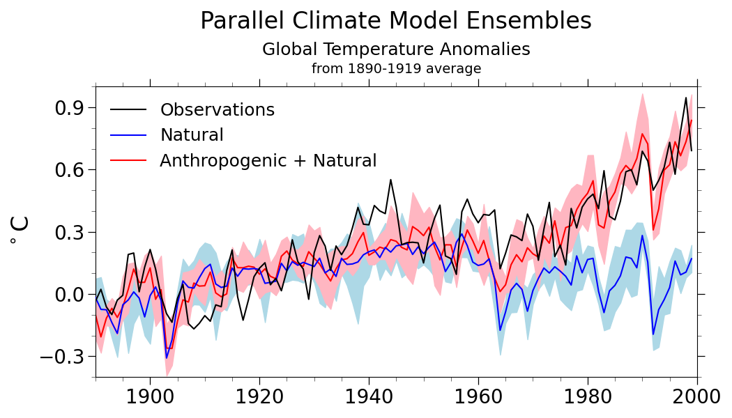
NCL_xy_18.py#

This script illustrates the following concepts:

Filling the area between two curves in an XY plot
Labeling the bottom X axis with years
Drawing a main title on three separate lines
Calculating a weighted average
Changing the size/shape of an XY plot using viewport resources
Manually creating a legend
Overlaying XY plots on each other
Maximizing plots after they’ve been created

See following URLs to see the reproduced NCL plot & script:

Original NCL script: https://www.ncl.ucar.edu/Applications/Scripts/xy_18.ncl
Original NCL plot: https://www.ncl.ucar.edu/Applications/Images/xy_18_lg.png

Import packages:

import numpy as np
import xarray as xr
from matplotlib import pyplot as plt

import geocat.datafiles as gdf
import geocat.viz as gv

Read in data:#

Open files and read in monthly data

Xarray’s open_mfdataset (open multi-file dataset) method will attempt to merge all of the individual datasets (i.e., NetCDF files) into one single Xarray Dataset. The concat_dim and combine keyword arguments to this method give you control over how this merging takes place (see the Xarray documentation for more information).

In the below example, each NetCDF file represents the same variables and coordinates, but from a different ensemble member. There is no case (or ensemble) dimension explicitly declared in the files, so we use the concat_dim argument to state that we will create a new dimension called case that spans the ensemble members. Here, each file contains a TREFHT variable that depends upon dimensions (time, lat, lon) and coordinate variables time, lat and lon. After opening these files with open_mfdataset, the resulting Xarray Dataset will consist of a TREFHT variable that depends upon dimensions (case, time, lat, lon) and coordinate variables case, time, lat and lon.

NOTE: One of the files (TREFHT.B06.69.atm.1890-1999ANN.nc) contains a time coordinate variable with a calendar attribute having the value noleap (i.e., the “No leap year” non-standard calendar). The time coordinate variable in all of the other files do not have a calendar attribute at all. By default, when Xarray’s open_mfdataset reads each individual dataset, it will attempt to decode the time coordinate into an appropriate datetime object, so that you can then take advantage of Xarray’s (and Pandas’s) excellent time-series manipulation capabilities. However, due to the lacking calendar attribute in most of the files (which, according to CF conventions, defaults to the standard Gregorian calendar) and the noleap calendar attribute in one of the files, the time coordinate variable will be interpreted as “non-uniform” across all of the datasets. To fix this problem, we tell Xarray’s open_mfdataset function to not decode the time coordinate into datetime objects by passing the decode_times=False argument. Second, we pass a pre-processing function via the preprocess argument to open_mfdataset, telling Xarray to read each individual dataset from file (with the decode_times=False option) and then modify the resulting dataset according to the pre-processing function. In this case, the pre-processing function (assume_noleap_calendar) takes the single-file dataset, sets the calendar attribute of the time coordinate variable to noleap, and returns the decoded dataset (using the Xarray function decode_cf). Work-arounds like this are needed whenever you have “errors” or “inconsistancies” in your data.

# Define the xarray.open_mfdataset pre-processing function
# (Must take an xarray.Dataset as input and return an xarray.Dataset)
def assume_noleap_calendar(ds):
    ds.time.attrs['calendar'] = 'noleap'
    return xr.decode_cf(ds)


# Create a dataset for the "natural" (i.e., no anthropogenic effects) data
nfiles = [
    gdf.get("netcdf_files/TREFHT.B06.66.atm.1890-1999ANN.nc"),
    gdf.get("netcdf_files/TREFHT.B06.67.atm.1890-1999ANN.nc"),
    gdf.get("netcdf_files/TREFHT.B06.68.atm.1890-1999ANN.nc"),
    gdf.get("netcdf_files/TREFHT.B06.69.atm.1890-1999ANN.nc")
]
nds = xr.open_mfdataset(nfiles,
                        concat_dim='case',
                        combine='nested',
                        preprocess=assume_noleap_calendar,
                        decode_times=False)

# Create a dataset for the "natural + anthropogenic" data
vfiles = [
    gdf.get("netcdf_files/TREFHT.B06.61.atm.1890-1999ANN.nc"),
    gdf.get("netcdf_files/TREFHT.B06.59.atm.1890-1999ANN.nc"),
    gdf.get("netcdf_files/TREFHT.B06.60.atm.1890-1999ANN.nc"),
    gdf.get("netcdf_files/TREFHT.B06.57.atm.1890-1999ANN.nc")
]
vds = xr.open_mfdataset(vfiles,
                        concat_dim='case',
                        combine='nested',
                        preprocess=assume_noleap_calendar,
                        decode_times=False)

# Read the "weights" file
# (The xarray.Dataset.expand_dims call adds the longitude dimension to the
# dataset, which originally depends only upon the latitude dimension. This
# arguably makes computing the weighted means below more straight-forward.)
gds = xr.open_dataset(gdf.get("netcdf_files/gw.nc"))
gds = gds.expand_dims(dim={'lon': nds.lon})

Observations:#

Read in the observational data from an ASCII (text) file. Here, we use Numpy’s nice loadtxt method to read the data from the text file and return a Numpy array with float type. Then, we construct an Xarray DataArray explicitly, since the time values are not stored in the ASCII data file (we have to know them!).

obs_data = np.loadtxt(gdf.get("ascii_files/jones_glob_ann_2002.asc"),
                      dtype=float)
obs_time = xr.cftime_range('1856-07-16T22:00:00',
                           freq='365D',
                           periods=len(obs_data),
                           calendar='noleap')
obs = xr.DataArray(name='TREFHT', data=obs_data, coords=[('time', obs_time)])

NCL-based Weighted Mean Function:#

We define this function just for convenience. This is equivalent to how NCL computes the weighted mean.

def horizontal_weighted_mean(var, wgts):
    return (var * wgts).sum(dim=['lat', 'lon']) / wgts.sum(dim=['lat', 'lon'])

Natural data:#

We compute the weighted mean across the latitude and longitude dimensions (leaving only the case and time dimensions), and then we compute the anomaly measured from the average of the first 30 years.

gavn = horizontal_weighted_mean(nds["TREFHT"], gds["gw"])
gavan = gavn - gavn.sel(time=slice('1890', '1920')).mean(dim='time')

Natural + Anthropogenic data:#

We do the same thing for the “natural + anthropogenic” data.

gavv = horizontal_weighted_mean(vds["TREFHT"], gds["gw"])
gavav = gavv - gavv.sel(time=slice('1890', '1920')).mean(dim='time')

Observation data:#

We do the same thing for the observation data.

obs_avg = obs.sel(time=slice('1890', '1999')) - obs.sel(
    time=slice('1890', '1920')).mean(dim='time')

Calculate the ensemble Min. & Max. & Mean:#

Here we find the min, max, and mean along the case (i.e., ensemble) dimension (leaving only the time dimension) for both of our datasets. We compute the equivalent anomaly for the observations data.

gavan_min = gavan.min(dim='case')
gavan_max = gavan.max(dim='case')
gavan_avg = gavan.mean(dim='case')

gavav_min = gavav.min(dim='case')
gavav_max = gavav.max(dim='case')
gavav_avg = gavav.mean(dim='case')

Plot:#

# Generate figure (set its size (width, height) in inches) and axes
fig, ax = plt.subplots(figsize=(10.5, 6))

# We create the time axis data, not as datetime objects, but as just years
# The following line of code is equivalent to this:
#     time = [t.year for t in gavan.time.values]
# but it uses Xarray's convenient DatetimeAccessor functionality.
time = gavan.time.dt.year

# Plot data and add a legend
ax.plot(time, obs_avg, color='black', label='Observations', zorder=4)
ax.plot(time, gavan_avg, color='blue', label='Natural', zorder=3)
ax.plot(time, gavav_avg, color='red', label='Anthropogenic + Natural', zorder=2)
ax.legend(loc='upper left', frameon=False, fontsize=18)

# Use geocat.viz.util convenience function to add minor and major tick lines
gv.add_major_minor_ticks(ax,
                         x_minor_per_major=4,
                         y_minor_per_major=3,
                         labelsize=20)

# Use geocat.viz.util convenience function to set axes limits & tick values without calling several matplotlib functions
gv.set_axes_limits_and_ticks(ax,
                             xlim=(1890, 2000),
                             ylim=(-0.4, 1),
                             xticks=np.arange(1900, 2001, step=20),
                             yticks=np.arange(-0.3, 1, step=0.3))

# Set three titles on top of each other using axes title and texts
ax.set_title('Parallel Climate Model Ensembles', fontsize=24, pad=60.0)
ax.text(0.5,
        1.125,
        'Global Temperature Anomalies',
        fontsize=18,
        ha='center',
        va='center',
        transform=ax.transAxes)
ax.text(0.5,
        1.06,
        'from 1890-1919 average',
        fontsize=14,
        ha='center',
        va='center',
        transform=ax.transAxes)
ax.set_ylabel('$^\circ$C', fontsize=24)
ax.fill_between(time, gavan_min, gavan_max, color='lightblue', zorder=0)
ax.fill_between(time, gavav_min, gavav_max, color='lightpink', zorder=1)

# Show the plot
plt.tight_layout()
plt.show()

Total running time of the script: (0 minutes 8.102 seconds)

Gallery generated by Sphinx-Gallery

NCL_xy_18.py

Contents