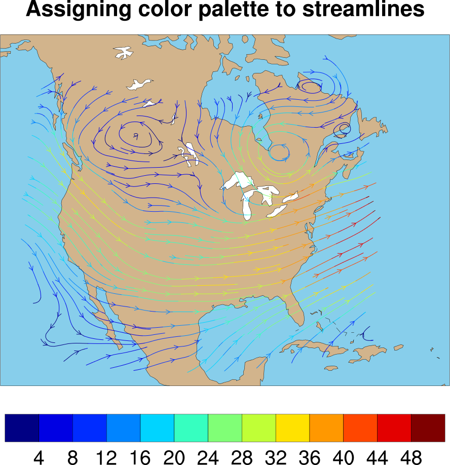
NCL_stream_9.py

This script illustrates the following concepts:

• Defining your own color map

• Applying a color map to a streamplot

• Using opacity to emphasize or subdue overlain features

See following URLs to see the reproduced NCL plot & script:

• Original NCL script: https://www.ncl.ucar.edu/Applications/Scripts/stream_9.ncl

• Original NCL plot: https://www.ncl.ucar.edu/Applications/Images/stream_9_1_lg.png

Import packages:

import numpy as np
import xarray as xr
import cartopy.crs as ccrs
import cartopy.feature as cfeature
import matplotlib.cm as cm
import matplotlib.pyplot as plt
import matplotlib.colors as colors
import matplotlib.colors as mcolors

import geocat.datafiles as gdf
import geocat.viz as gv

Make color map

colormap = colors.ListedColormap([
    'darkblue', 'mediumblue', 'blue', 'cornflowerblue', 'skyblue', 'aquamarine',
    'lime', 'greenyellow', 'gold', 'orange', 'orangered', 'red', 'maroon'
])

colorbounds = np.arange(0, 56, 4)

norm = mcolors.BoundaryNorm(colorbounds, colormap.N)

Read in data:

# Open a netCDF data file using xarray default engine and load the data into xarrays
ds1 = xr.open_dataset(gdf.get('netcdf_files/U500storm.cdf'))
ds2 = xr.open_dataset(gdf.get('netcdf_files/V500storm.cdf'))

Plot:

# Set figure
fig = plt.figure(figsize=(10, 10))

# Create first subplot on figure for map
ax = fig.add_axes([.1, .2, .8, .6],
                  projection=ccrs.LambertAzimuthalEqualArea(
                      central_longitude=-100, central_latitude=40),
                  frameon=False,
                  aspect='auto')

# Set axis projection
ax.set_extent([-128, -58, 18, 65], crs=ccrs.PlateCarree())

# Add ocean, lakes, land features, and coastlines to map
ax.add_feature(cfeature.OCEAN, color='lightblue')
ax.add_feature(cfeature.LAKES, color='white', edgecolor='black')
ax.add_feature(cfeature.LAND, color='tan')
ax.coastlines()

# Extract streamline data from initial timestep
U = ds1.u.isel(timestep=0)
V = ds2.v.isel(timestep=0)

# Calculate magnitude data
magnitude = np.sqrt(np.square(U.data) + np.square(V.data))

# Plot streamline data
streams = ax.streamplot(U.lon,
                        U.lat,
                        U.data,
                        V.data,
                        transform=ccrs.PlateCarree(),
                        arrowstyle='->',
                        linewidth=1,
                        density=2.0,
                        color=magnitude,
                        cmap=colormap)

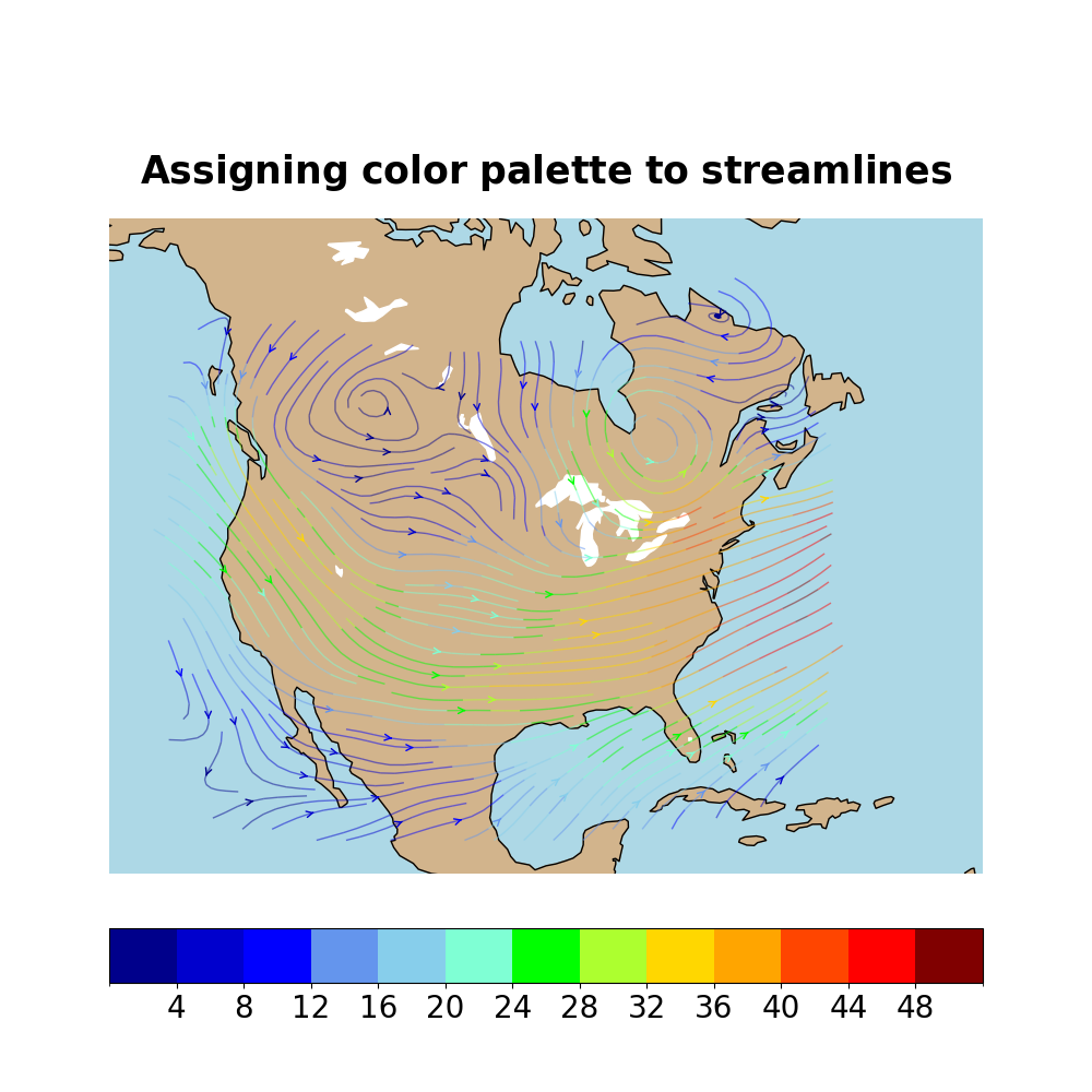
# Set streamlines and arrows to partially transparent
streams.lines.set_alpha(.5)
streams.arrows.set_alpha(.5)

# Create second subplot on figure for colorbar
ax2 = fig.add_axes([.1, .1, .8, .05])

# Set title of plot
# Make title font bold using r"$\bf{_______}$" formatting
gv.set_titles_and_labels(ax,
                         maintitle=r"$\bf{Assigning}$" + " " + r"$\bf{color}$" +
                         " " + r"$\bf{palette}$" + " " + r"$\bf{to}$" + " " +
                         r"$\bf{streamlines}$",
                         maintitlefontsize=25)

# Plot colorbar on subplot
cb = fig.colorbar(cm.ScalarMappable(cmap=colormap, norm=norm),
                  cax=ax2,
                  boundaries=colorbounds,
                  ticks=np.arange(4, 52, 4),
                  spacing='uniform',
                  orientation='horizontal')

# Change size of colorbar tick font
ax2.tick_params(labelsize=20)

plt.show()