

Note
Go to the end to download the full example code.
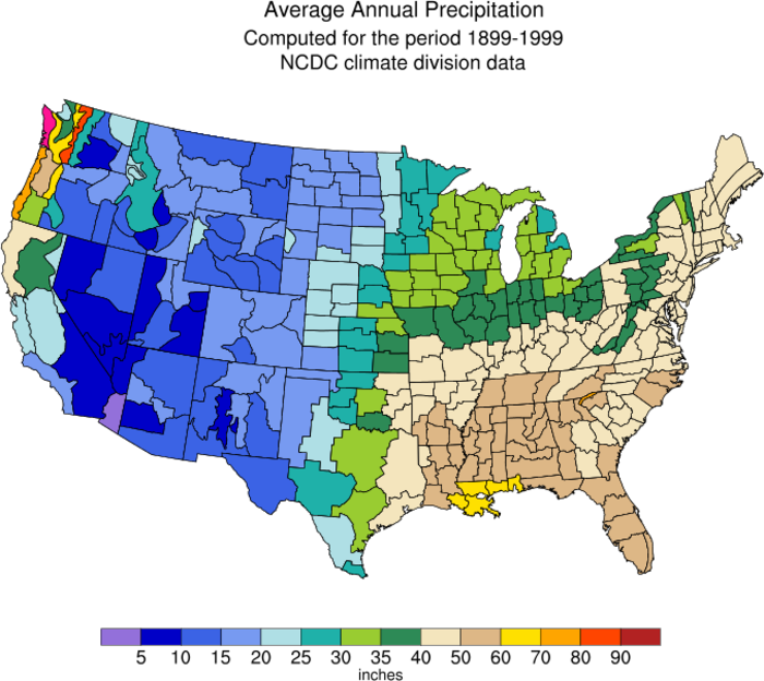
NCL_polyg_2.py#
- Concepts illustrated:
Drawing a Lambert Conformal U.S. map color-coded by climate divisions
Color-coding climate divisions based on precipitation values
Drawing the climate divisions of the U.S.
Zooming in on a particular area on a Lambert Conformal map
Drawing a border around filled polygons
Masking the ocean in a map plot
Masking land in a map plot
Increasing the font size of text
Adding text to a plot
Drawing a custom labelbar on a map
Creating a red-yellow-blue color map
- See following URLs to see the reproduced NCL plot & script:
Original NCL script: https://www.ncl.ucar.edu/Applications/Scripts/polyg_2.ncl
Original NCL plot: https://www.ncl.ucar.edu/Applications/Images/polyg_2_lg.png
Import packages:
import xarray as xr
import cartopy.crs as ccrs
import matplotlib.pyplot as plt
import matplotlib.colors as colors
import matplotlib.cm as cm
import geocat.viz as gv

import geocat.datafiles as gdf
import cartopy.io.shapereader as shpreader
import shapely.geometry as sgeom
from mpl_toolkits.axes_grid1.inset_locator import inset_axes
Read in data
# Open climate division datafile and add to xarray
ds = xr.open_dataset(
    gdf.get("netcdf_files/climdiv_prcp_1899-1999.nc"), decode_times=False
)
Initialize color map and bounds for each color
colormap = colors.ListedColormap(
[
'mediumpurple',
'mediumblue',
'royalblue',
'cornflowerblue',
'lightblue',
'lightseagreen',
'yellowgreen',
'green',
'wheat',
'tan',
'gold',
'orange',
'red',
'firebrick',
]
)
# Values represent average number of inches of rain
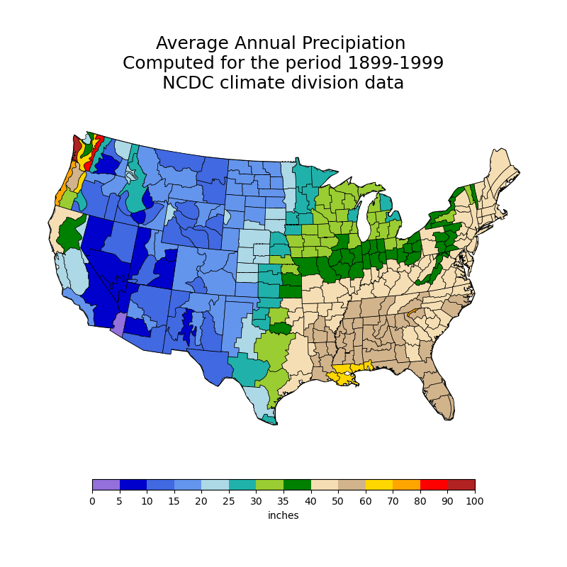
colorbounds = [0, 5, 10, 15, 20, 25, 30, 35, 40, 50, 60, 70, 80, 90, 100]
Define helper function to determine which color to fill the divisions based on precipitation data
def findDivColor(colorbounds, pdata):
    for x in range(len(colorbounds)):
        if pdata >= colorbounds[len(colorbounds) - 1]:
            return colormap.colors[x - 1]
        if pdata >= colorbounds[x]:
            continue
        else:
            # Index is 'x-1' because colorbounds is one item longer than colormap
            return colormap.colors[x - 1]
Create plot
# Create plot figure
fig = plt.figure(figsize=(8, 8))

# Add axes for lambert conformal map
# Set dimensions of axes with [X0, Y0, width, height] argument. Each value is a fraction of total figure size.
ax = plt.axes([0.05, -0.05, 0.9, 1], projection=ccrs.LambertConformal(), frameon=False)

# Set latitude and longitude extent of map
ax.set_extent([-119, -74, 18, 50], ccrs.Geodetic())

# Set shape name of map (which depicts the United States)
shapename = 'admin_1_states_provinces_lakes'
states_shp = shpreader.natural_earth(
    resolution='110m', category='cultural', name=shapename
)

# Set title and title fontsize of plot using gv function instead of matplotlib function call
gv.set_titles_and_labels(
    ax,
    maintitle="Average Annual Precipiation \n Computed for the period 1899-1999 \n NCDC climate division data \n",
    maintitlefontsize=18,
)

# Add outlines of each state within the United States
for state in shpreader.Reader(states_shp).geometries():
    facecolor = 'white'
    edgecolor = 'black'

    ax.add_geometries(
        [state], ccrs.PlateCarree(), facecolor=facecolor, edgecolor=edgecolor
    )

# For each variable (climate division) in data set, create outline on map and fill with random color
for varname, da in ds.data_vars.items():
    # This condition is included because first item in xarray only has one attribute, 'current date'
    if hasattr(da, 'state_name'):
        # Get number of years of data by dividing number of months recorded (length of array) by 12 (12 months per year)
        numYears = len(da.values) / 12

        # Get precipitation data for each climate division:
        # Rather than looping through the whole array to find the sum of each 12 values (a year's worth of data),
        # adding each sum to an array, and then finding the average of the values in the array, as seen in the NCL
        # script, the one-line python method involves summing the dataset values and then dividing it by numYears (calculated in line 99)
        precipitationdata = sum(da.values) / numYears

        # Get borders of each climate division
        lat = da.lat
        lon = da.lon

        # Get color of climate division
        color = findDivColor(colorbounds, precipitationdata)

        # Use "shapely geometry" module to create division outlines from lat/lon coordinates
        track = sgeom.LineString(zip(lon, lat))

        # Add division outlines to map
        im = ax.add_geometries(
            [track],
            ccrs.PlateCarree(),
            facecolor=color,
            edgecolor='black',
            linewidths=0.5,
        )

# Create and plot colorbar

# Map colors to bounds
norm = colors.BoundaryNorm(colorbounds, colormap.N)

# Add inset axes (axes within pre-existing axes) to hold colorbar
axins1 = inset_axes(ax, width="75%", height="3%", loc='lower center')

# Add colorbar to plot
cb = fig.colorbar(
    cm.ScalarMappable(cmap=colormap, norm=norm),
    cax=axins1,
    boundaries=colorbounds,
    ticks=colorbounds,
    spacing='uniform',
    orientation='horizontal',
    label='inches',
)

plt.show()
/home/docs/checkouts/readthedocs.org/user_builds/geocat-examples/conda/latest/lib/python3.14/site-packages/cartopy/io/__init__.py:242: DownloadWarning: Downloading: https://naturalearth.s3.amazonaws.com/110m_cultural/ne_110m_admin_1_states_provinces_lakes.zip
  warnings.warn(f'Downloading: {url}', DownloadWarning)
Total running time of the script: (0 minutes 2.861 seconds)