

Note
Go to the end to download the full example code.
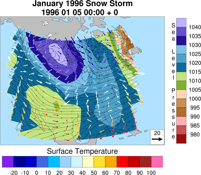
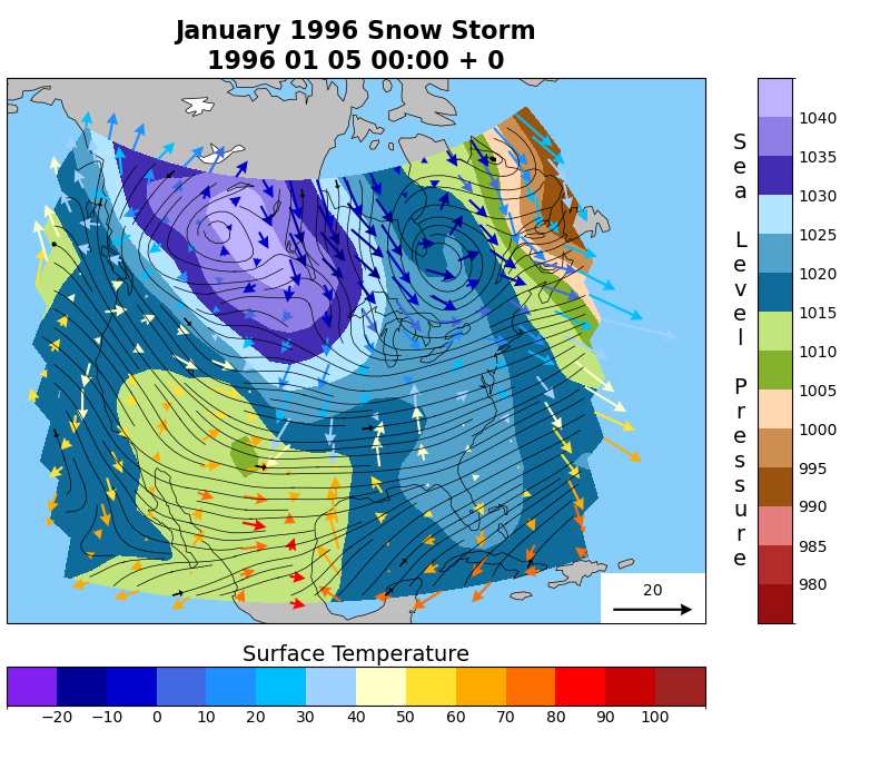
NCL_overlay_6.py#
- This script illustrates the following concepts:
Overlaying filled contours, streamlines, and vectors over the same map
Adding various map elements to a figure
Using inset_axes() to create additional axes for color bars
Creating custom label formats for colorbars
Creating a quiverkey
Assigning a colormap to contour and quiver plots
Add arrows to streamlines
Using zorder to specify the order in which elements will be drawn
- See following URLs to see the reproduced NCL plot & script:
Original NCL script: https://www.ncl.ucar.edu/Applications/Scripts/overlay_6.ncl
Original NCL plots: https://www.ncl.ucar.edu/Applications/Images/overlay_6_lg.png
- Differences between NCL example and this one:
In the NCL version of this plot the vectors for the winds are nearly uniform in length. Given the reference vector in that figure, the wind speeds appear to be near 20 units. A histogram reveals that this is not a true representation of the data as the magnitudes of the majority of wind vectors are between 3 and 6 units with only a handful being greater than 13 and only one near 20. Because of this, we have chosen not to manipulate the vector glyphs to appear more uniform as this would poorly represent the data and be misleading. The lengths of the vectors in this examples are proportional to the wind magnitudes where in the NCL examples they are not, which is why the reference vector in this Python example is longer than the NCL example and why the lengths vary more between the minimum and maximum wind speeds.
Import packages:
import numpy as np
import xarray as xr
import matplotlib.pyplot as plt
import matplotlib.patches as mpatches
from mpl_toolkits.axes_grid1.inset_locator import inset_axes
import cartopy.crs as ccrs
import cartopy.feature as cfeature
import matplotlib.colors as mcolors

import geocat.datafiles as gdf
import cmaps
Read in data:
# Open a netCDF data file using xarray default engine and load the data into xarrays
uf = xr.open_dataset(gdf.get("netcdf_files/Ustorm.cdf"))
vf = xr.open_dataset(gdf.get("netcdf_files/Vstorm.cdf"))
pf = xr.open_dataset(gdf.get("netcdf_files/Pstorm.cdf"))
tf = xr.open_dataset(gdf.get("netcdf_files/Tstorm.cdf"))
u500f = xr.open_dataset(gdf.get("netcdf_files/U500storm.cdf"))
v500f = xr.open_dataset(gdf.get("netcdf_files/V500storm.cdf"))

p = pf.p.isel(timestep=0, drop=True)
t = tf.t.isel(timestep=0, drop=True)
u = uf.u.isel(timestep=0, drop=True)
v = vf.v.isel(timestep=0, drop=True)
u500 = u500f.u.isel(timestep=0, drop=True)
v500 = v500f.v.isel(timestep=0, drop=True)
time = vf.timestep

# Convert Pa to hPa
p = p / 100
# Convert K to F
t = (t - 273.15) * 9 / 5 + 32
Create plot:
fig = plt.figure(figsize=(8, 7))
proj = ccrs.LambertAzimuthalEqualArea(central_longitude=-100, central_latitude=40)

# Set axis projection
ax = plt.axes([0, 0.2, 0.8, 0.7], projection=proj)
# Create inset axes for color bars
cax1 = inset_axes(
    ax,
    width='5%',
    height='100%',
    loc='lower right',
    bbox_to_anchor=(0.125, 0, 1, 1),
    bbox_transform=ax.transAxes,
    borderpad=0,
)

cax2 = inset_axes(
    ax,
    width='100%',
    height='7%',
    loc='lower left',
    bbox_to_anchor=(0, -0.15, 1, 1),
    bbox_transform=ax.transAxes,
    borderpad=0,
)

# Set extent to include roughly the United States
ax.set_extent((-128, -58, 18, 65), crs=ccrs.PlateCarree())

#
# Add map features
#
# Using the zorder keyword, we can specify the order of the layering. Lower
# numbers are plotted before higher ones. For example, the coastlines have
# zorder=2 while the filled contours have zorder=1. This will draw the
# coastlines on top of the filled contours.
transparent = (0, 0, 0, 0)  # RGBA value for a transparent color for lakes
ax.add_feature(cfeature.OCEAN, color='lightskyblue', zorder=0)
ax.add_feature(cfeature.LAND, color='silver', zorder=0)
ax.add_feature(
    cfeature.LAKES, linewidth=0.5, edgecolor=transparent, facecolor='white', zorder=0
)
ax.add_feature(
    cfeature.LAKES, linewidth=0.5, edgecolor='black', facecolor=transparent, zorder=2
)
ax.add_feature(cfeature.COASTLINE, linewidth=0.5, zorder=2)

#
# Plot pressure level contour
#
p_cmap = cmaps.StepSeq25
pressure = p.plot.contourf(
    ax=ax,
    transform=ccrs.PlateCarree(),
    cmap=p_cmap,
    levels=np.arange(975, 1050, 5),
    add_colorbar=False,
    add_labels=False,
    zorder=1,
)
plt.colorbar(pressure, cax=cax1, ticks=np.arange(980, 1045, 5))

# Format color bar label
cax1.yaxis.set_label_text(
    label='\n'.join('Sea Level Pressure'), fontsize=14, rotation=0
)
cax1.yaxis.set_label_coords(-0.5, 0.9)
cax1.tick_params(size=0)

#
# Overlay streamlines
#
with np.errstate(
    invalid='ignore'
):  # Indeed not needed, just to get rid of warnings about numpy's NaN comparisons
    streams = ax.streamplot(
        u500.lon,
        u500.lat,
        u500.data,
        v500.data,
        transform=ccrs.PlateCarree(),
        color='black',
        arrowstyle='-',
        linewidth=0.5,
        density=2,
        zorder=5,
    )

# Divide streamlines into segments
seg = streams.lines.get_segments()
# Determine how many arrows on each streamline, the placement, and angles of the arrows
period = 7
arrow_x = np.array([seg[i][0, 0] for i in range(0, len(seg), period)])
arrow_y = np.array([seg[i][0, 1] for i in range(0, len(seg), period)])
arrow_dx = np.array([seg[i][1, 0] - seg[i][0, 0] for i in range(0, len(seg), period)])
arrow_dy = np.array([seg[i][1, 1] - seg[i][0, 1] for i in range(0, len(seg), period)])
# Add arrows to streamlines
q = ax.quiver(
    arrow_x,
    arrow_y,
    arrow_dx,
    arrow_dy,
    color='black',
    angles='xy',
    scale=1,
    units='y',
    minshaft=3,
    headwidth=4,
    headlength=2,
    headaxislength=2,
    zorder=5,
)

#
# Overlay wind vectors
#
# First thin the data so the vector grid is less cluttered
lon_size = u['lon'].size
lat_size = u['lat'].size

x = u['lon'].data[0:lon_size:2]
y = u['lat'].data[0:lat_size:2]
u = u.data[0:lat_size:2, 0:lon_size:2]
v = v.data[0:lat_size:2, 0:lon_size:2]
t = t.data[0:lat_size:2, 0:lon_size:2]

# Import and modify color map for vectors
wind_cmap = cmaps.amwg_blueyellowred
bounds = np.arange(-30, 120, 10)  # Sets where boundaries on color map will be
norm = mcolors.BoundaryNorm(bounds, wind_cmap.N)  # Assigns colors to values
# Draw wind vectors
with np.errstate(
    invalid='ignore'
):  # Indeed not needed, just to get rid of warnings about numpy's NaN comparisons
    Q = ax.quiver(
        x,
        y,
        u,
        v,
        t,
        transform=ccrs.PlateCarree(),
        norm=norm,
        headwidth=5,
        cmap=wind_cmap,
        zorder=4,
    )

# Add color bar
plt.colorbar(Q, cax=cax2, ticks=np.arange(-20, 110, 10), orientation='horizontal')

# Format color bar label
cax2.xaxis.set_label_text(label='Surface Temperature', fontsize=14)
cax2.xaxis.set_label_position('top')
cax2.tick_params(size=0)

# Add quiverkey and white patch behind it
ax.add_patch(
    mpatches.Rectangle(
        xy=[0.85, 0],
        width=0.15,
        height=0.0925,
        facecolor='white',
        transform=ax.transAxes,
        zorder=3,
    )
)
ax.quiverkey(Q, 0.925, 0.025, 20, label='20', zorder=4)

# Add title
ax.set_title(
    'January 1996 Snow Storm\n1996 01 05 00:00 + 0', fontweight='bold', fontsize=16
)

plt.show()
Total running time of the script: (0 minutes 3.747 seconds)