NCL_WRF_interp_3.py

This script illustrates the following concepts:

• Interpolating a vertical cross-section from a 3D WRF-ARW field.

• Recombining two datasets into one usable form

• Following best practices when choosing a colormap. More information on colormap best practices can be found here.

See following URLs to see the reproduced NCL plot & script:

• Original NCL script: https://www.ncl.ucar.edu/Applications/Scripts/wrf_interp_3.ncl

• Original NCL plot: https://www.ncl.ucar.edu/Applications/Images/wrf_interp_3_lg.png

Import packages

from netCDF4 import Dataset
import numpy as np
import matplotlib.pyplot as plt
import xarray as xr
import os

from wrf import to_np, getvar, CoordPair, vertcross, latlon_coords
import geocat.datafiles as gdf
import geocat.viz as gv

Read in the data

# Specify the necessary variables needed from the data set in order to use 'z' and 'QVAPOR'
toinclude = ['PH', 'P', 'HGT', 'PHB', 'QVAPOR']
# Read in necessary datasets
ds = xr.open_mfdataset(
    [
        gdf.get('netcdf_files/wrfout_d03_2012-04-22_23_00_00_Z.nc'),
        gdf.get('netcdf_files/wrfout_d03_2012-04-22_23_00_00_QV.nc'),
    ]
)

# specify a unique output file name to use to read in combined dataset later
file3 = 'wrfout_d03_2012-04-22_23.nc'
mrg = ds[toinclude].to_netcdf(file3)

# Read in the data and extract variables
wrfin = Dataset(('wrfout_d03_2012-04-22_23.nc'))

z = getvar(wrfin, "z")
qv = getvar(wrfin, "QVAPOR")
# Pull lat/lon coords from QVAPOR data using wrf-python tools
lats, lons = latlon_coords(qv)

/home/docs/checkouts/readthedocs.org/user_builds/geocat-examples/checkouts/latest/Gallery/WRF/NCL_wrf_interp_3.py:34: FutureWarning: In a future version of xarray the default value for compat will change from compat='no_conflicts' to compat='override'. This is likely to lead to different results when combining overlapping variables with the same name. To opt in to new defaults and get rid of these warnings now use `set_options(use_new_combine_kwarg_defaults=True) or set compat explicitly.
  ds = xr.open_mfdataset(
/home/docs/checkouts/readthedocs.org/user_builds/geocat-examples/checkouts/latest/Gallery/WRF/NCL_wrf_interp_3.py:34: FutureWarning: In a future version of xarray the default value for compat will change from compat='no_conflicts' to compat='override'. This is likely to lead to different results when combining overlapping variables with the same name. To opt in to new defaults and get rid of these warnings now use `set_options(use_new_combine_kwarg_defaults=True) or set compat explicitly.
  ds = xr.open_mfdataset(

Create vertical cross section using wrf-python tools

# Define start and stop coordinates for cross section
start_point = CoordPair(lat=38, lon=-118)
end_point = CoordPair(lat=40, lon=-115)

qv_cross = vertcross(
    qv, z, wrfin=wrfin, start_point=start_point, end_point=end_point, latlon=True
)

# Close 'wrfin' to prevent PermissionError if code is run more than once locally
wrfin.close()
# Remove created wrfout file from local directory
os.remove('wrfout_d03_2012-04-22_23.nc')

Plot the data

fig = plt.figure(figsize=(10, 8))
ax = plt.axes()

# Set the x-ticks to use latitude and longitude labels.
coord_pairs = to_np(qv_cross.coords["xy_loc"])
x_ticks = np.arange(coord_pairs.shape[0])

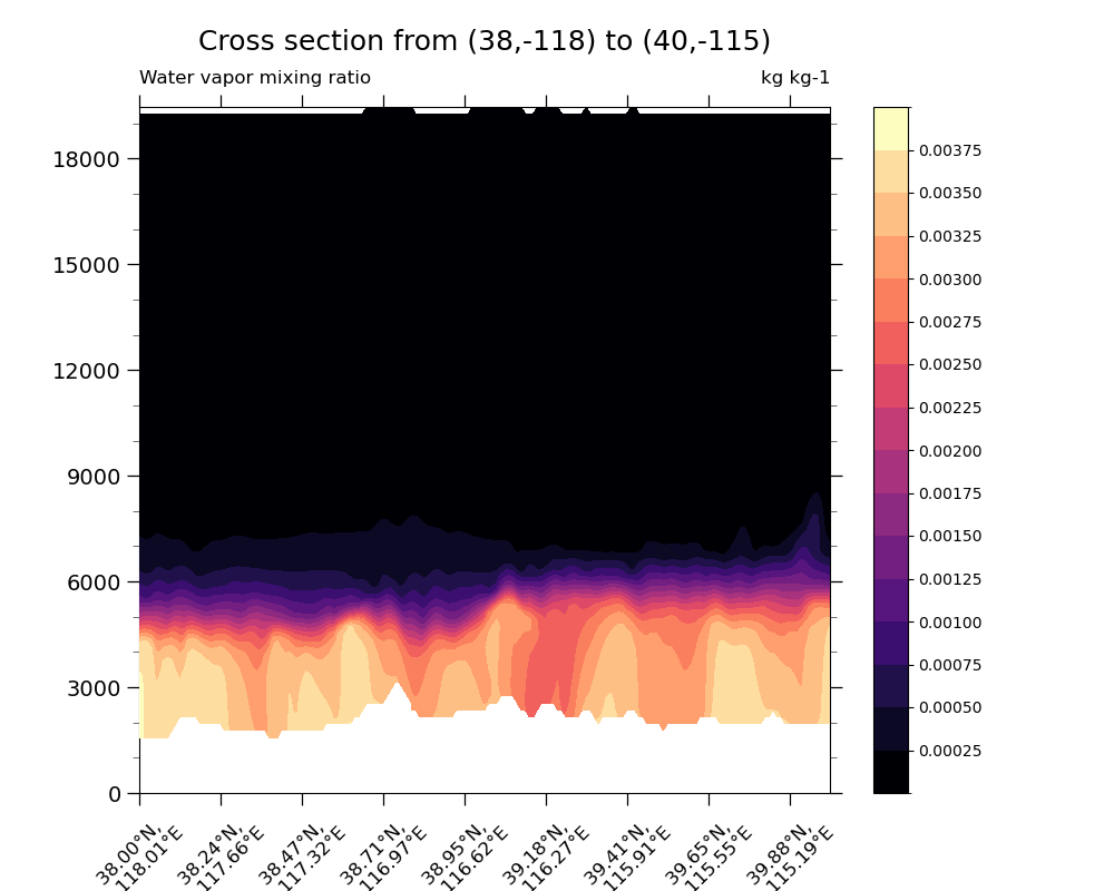
# Plot filled contours
qv_contours = qv_cross.plot.contourf(
    ax=ax,
    levels=17,
    cmap='magma',
    vmin=0,
    vmax=0.004,
    zorder=4,
    add_labels=False,
    add_colorbar=False,
    yticks=np.arange(0, 20000, 3000),
    xticks=x_ticks[::20],
)
# Add colorbar
plt.colorbar(qv_contours, ax=ax, ticks=np.arange(0.00025, 0.004, 0.00025))

# Add minor ticks to the yaxis
gv.add_major_minor_ticks(ax=ax, x_minor_per_major=1, y_minor_per_major=3, labelsize=14)

# Format the xtick labels
x_labels = [
    pair.latlon_str(fmt="{:.2f}\N{DEGREE SIGN}N, \n {:.2f}\N{DEGREE SIGN}E")
    for pair in to_np(coord_pairs)
]
ax.set_xticklabels(x_labels[::20], rotation=45, fontsize=12)

# Set the plot titles
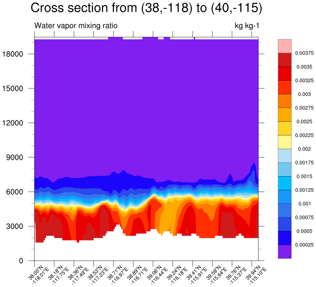
plt.title("Cross section from (38,-118) to (40,-115)", fontsize=18, y=1.07)
plt.title('Water vapor mixing ratio', loc='left', y=1.02)
plt.title('kg kg-1', loc='right', y=1.02)

plt.show()