NCL_mask_5.py

This script illustrates the following concepts:

• Using cartopy.feature options to display map information

• Paneling two plots on a page with ‘subplots’ command

• Drawing contours

• Drawing contours over land only

• Using draw order resources to mask areas in a plot

• Adding a color bar

• Following best practices when choosing a colormap. More information on colormap best practices can be found here.

See following URLs to see the reproduced NCL plot & script:

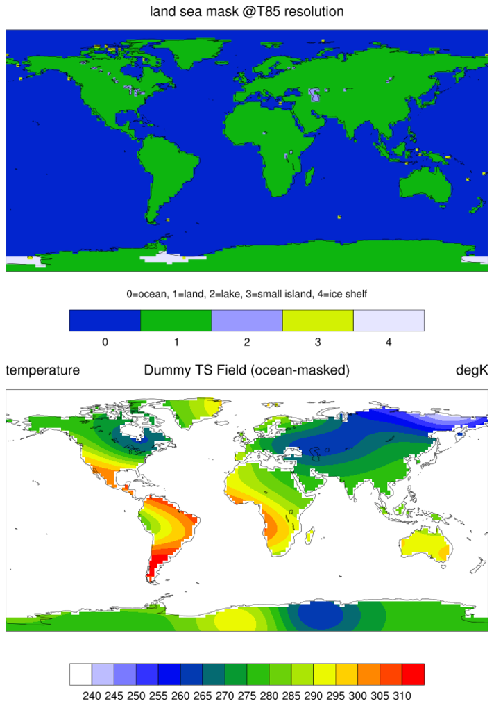
• Original NCL script: https://www.ncl.ucar.edu/Applications/Scripts/mask_5.ncl

• Original NCL plot: https://www.ncl.ucar.edu/Applications/Images/mask_5_lg.png

Import packages:

import numpy as np
import xarray as xr
import cartopy.crs as ccrs
import matplotlib.pyplot as plt
import cartopy.feature as cfeature
import matplotlib.patches as mpatches

import geocat.viz as gv
import geocat.datafiles as gdf

Read in Data

# Open a netCDF data file using xarray default engine and load the data into xarrays
ds = xr.open_dataset(gdf.get("netcdf_files/atmos.nc"), decode_times=False)
t = ds.TS.isel(time=0)

# Fix the artifact of not-shown-data around 0 and 360-degree longitudes
wrap_t = gv.xr_add_cyclic_longitudes(t, "lon")

Plot:

fig = plt.figure(figsize=(10, 15))

# Plot first plot
# Generate axes using Cartopy, draw coastlines, and add other map features
ax = plt.subplot(2, 1, 1, projection=ccrs.PlateCarree())
ax.coastlines(linewidths=0.5)
ax.add_feature(cfeature.LAND, color="green")
ax.add_feature(cfeature.LAKES, color="plum")
ax.add_feature(cfeature.OCEAN, color="blue")

# Cartopy does not currently have a feature that separates island land from
# main land. There is also no feature to add ice shelf data to a projection.
# This addition would require another data set to specify area encompassed
# by an ice shelf in a region.

# Create label names and define colors for the legend
land = mpatches.Rectangle((0, 0), 1, 1, facecolor="green")
lakes = mpatches.Rectangle((0, 0), 1, 1, facecolor="plum")
ocean = mpatches.Rectangle((0, 0), 1, 1, facecolor="blue")

labels = ['Land ', 'Lakes', 'Ocean']

# Add a legend to plot
plt.legend([land, lakes, ocean],
           labels,
           loc='lower center',
           bbox_to_anchor=(0.5, -0.2),
           ncol=3)

# Use geocat.viz.util convenience function to set titles and labels without
# calling several matplotlib functions
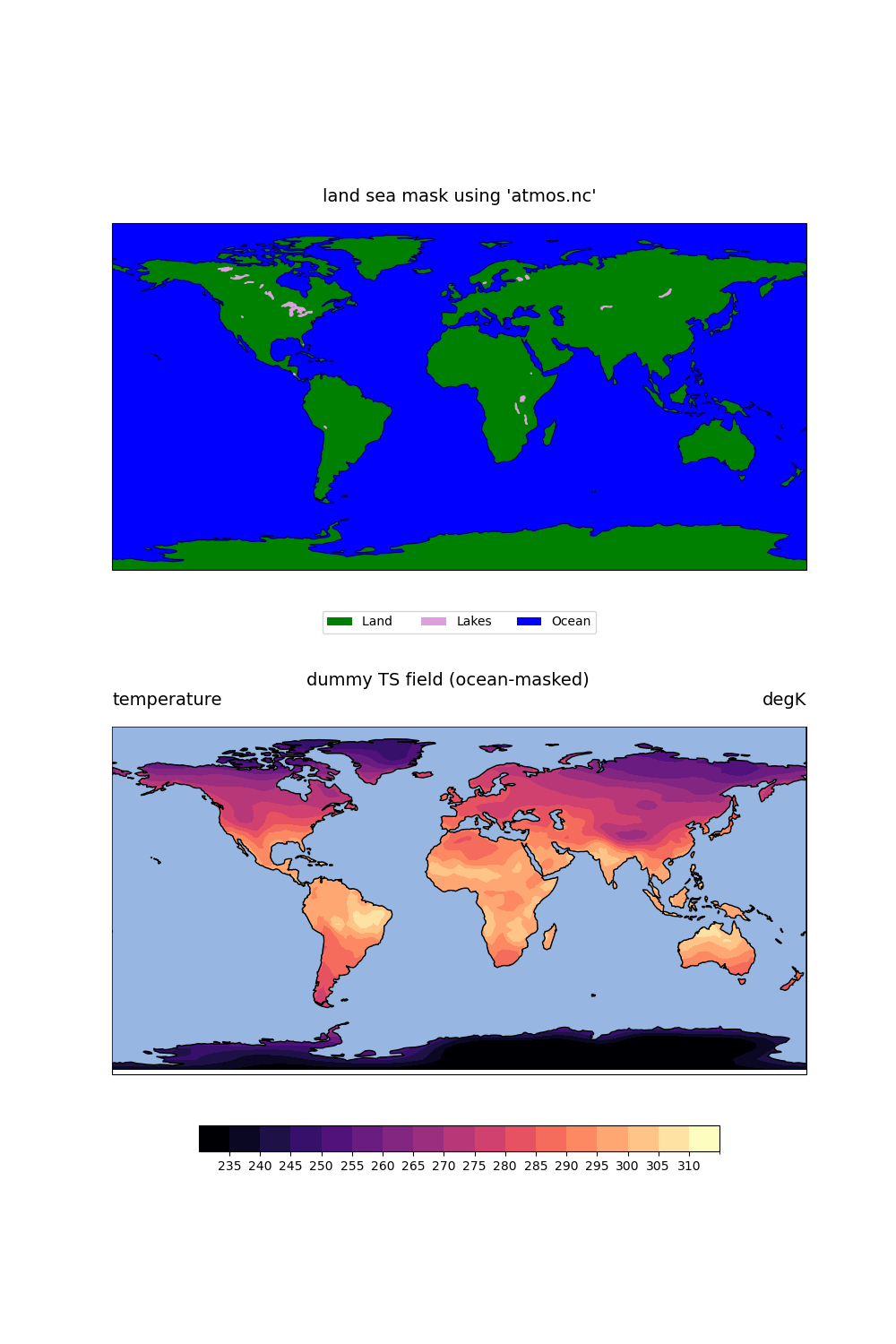
gv.set_titles_and_labels(ax,
                         maintitle="land sea mask using 'atmos.nc'",
                         maintitlefontsize=14)

# Plot second plot
ax1 = plt.subplot(2, 1, 2, projection=ccrs.PlateCarree())
ax1.set_extent([-180, 180, -90, 90], ccrs.PlateCarree())
ax1.coastlines(linewidths=0.5)

plt.suptitle("dummy TS field (ocean-masked)", x=0.5, y=0.5, fontsize=14)

# Contourf-plot data
contour = wrap_t.plot.contourf(ax=ax1,
                               transform=ccrs.PlateCarree(),
                               vmin=235,
                               vmax=315,
                               levels=17,
                               cmap='magma',
                               add_colorbar=False)

# Add colorbar to bottom of plot
cbar = plt.colorbar(contour,
                    ax=ax1,
                    orientation='horizontal',
                    shrink=0.75,
                    pad=0.11,
                    extendrect=True,
                    extendfrac='auto',
                    use_gridspec=False,
                    ticks=np.arange(235, 315, 5))

cbar.ax.tick_params(labelsize=10)

# Mask ocean data by changing adding ocean feature and changing its zorder
ax1.add_feature(cfeature.OCEAN, zorder=10, edgecolor='k')

# Use geocat.viz.util convenience function to set titles and labels without
# calling several matplotlib functions
gv.set_titles_and_labels(ax1,
                         maintitle="",
                         maintitlefontsize=14,
                         righttitle="degK",
                         righttitlefontsize=14,
                         lefttitle="temperature",
                         lefttitlefontsize=14)

plt.show()