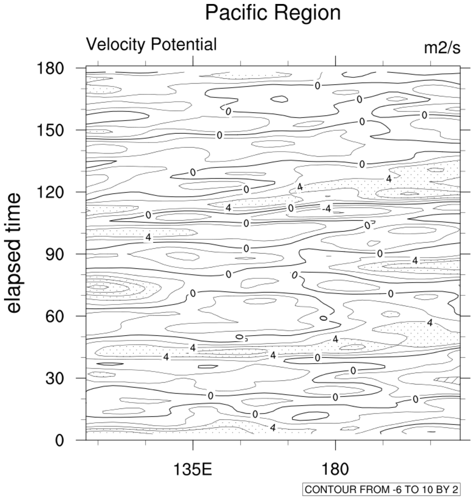
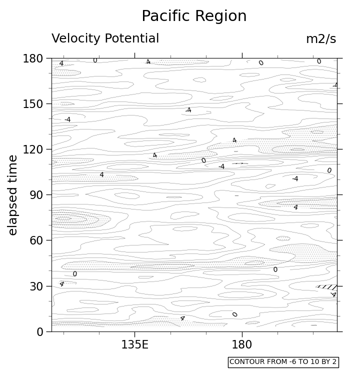
NCL_hov_3.py

This script illustrates the following concepts:

• Creating a Hovmueller plot

• Hatching fill between contours

See following URLs to see the reproduced NCL plot & script:

• Original NCL script: https://www.ncl.ucar.edu/Applications/Scripts/hov_3.ncl

• Original NCL plot: https://www.ncl.ucar.edu/Applications/Images/hov_3_lg.png

Import packages:

import numpy as np
import xarray as xr

import matplotlib.pyplot as plt

import geocat.datafiles as gdf
import geocat.viz as gv

Read in data:

# Open a netCDF data file using xarray default engine
# and load the data into xarrays
ds = xr.open_dataset(gdf.get('netcdf_files/chi200_ud_smooth.nc'))

lon = ds.lon
times = ds.time
scale = 1000000
chi = ds.CHI
chi = chi / scale

/home/docs/checkouts/readthedocs.org/user_builds/geocat-examples/checkouts/latest/Gallery/Contours/NCL_hov_3.py:29: FutureWarning: In a future version of xarray decode_timedelta will default to False rather than None. To silence this warning, set decode_timedelta to True, False, or a 'CFTimedeltaCoder' instance.
  ds = xr.open_dataset(gdf.get('netcdf_files/chi200_ud_smooth.nc'))

Plot:

# Initialize figure and axis
fig, ax = plt.subplots(figsize=(7, 7.5))

# Fill area between level 4 contours and level 10 contours with dot hatching
cf = ax.contourf(lon, times, chi, levels=[4, 12], colors='None', hatches=['....'])

# Make all dot-filled areas light gray so contour lines are still visible
cf.set_edgecolor('lightgray')
cf.set_linewidth(0.0)

# Fill area at the lowest contour level, -6, with line hatching
cf = ax.contourf(lon, times, chi, levels=[-7, -6], colors='None', hatches=['///'])

# Draw contour lines at levels [-6, -4, -2, 0, 2, 4, 6, 8, 10]
cs = ax.contour(
    lon,
    times,
    chi,
    levels=np.arange(-6, 12, 2),
    colors='black',
    linestyles="-",
    linewidths=[0.2, 0.2, 0.2, 1, 0.2, 0.2, 0.2, 0.2, 0.2],
)

# Label the contour levels -4, 0, and 4
cl = ax.clabel(cs, fmt='%d', levels=[-4, 0, 4])

# Use geocat.viz.util convenience function to set axes limits & tick values
gv.set_axes_limits_and_ticks(
    ax,
    xlim=[100, 220],
    ylim=[0, 1.55 * 1e16],
    xticks=[135, 180],
    yticks=np.linspace(0, 1.55 * 1e16, 7),
    xticklabels=['135E', '180'],
    yticklabels=np.linspace(0, 180, 7, dtype='int'),
)

# Use geocat.viz.util convenience function to add minor and major tick lines
gv.add_major_minor_ticks(ax, x_minor_per_major=3, y_minor_per_major=3, labelsize=16)

# Use geocat.viz.util convenience function to add titles
gv.set_titles_and_labels(
    ax,
    maintitle="Pacific Region",
    maintitlefontsize=20,
    lefttitle="Velocity Potential",
    lefttitlefontsize=18,
    righttitle="m2/s",
    righttitlefontsize=18,
    ylabel="elapsed time",
    labelfontsize=18,
)

# Add lower text box
ax.text(
    1,
    -0.12,
    "CONTOUR FROM -6 TO 10 BY 2",
    horizontalalignment='right',
    transform=ax.transAxes,
    bbox=dict(boxstyle='square, pad=0.25', facecolor='white', edgecolor='black'),
)

plt.tight_layout()
plt.show()