

Note
Go to the end to download the full example code.
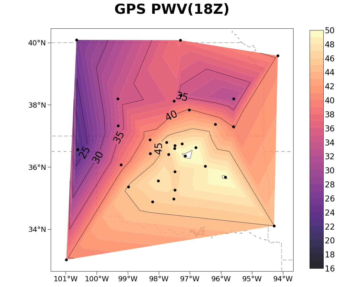
NCL_station_1.py#
- This script illustrates the following concepts:
Using pandas package to read in ascii file with several columns of data
Using tricontour and tricontourf function from matplotlib package to contour one-dimensional X, Y, Z data
Drawing lat/lon locations as filled dots
Controlling which contour lines get drawn
Using alpha parameter to emphasize or subdue overlain features
Using a different color scheme to follow best practices for visualizations
- See following URLs to see the reproduced NCL plot & script:
Original NCL script: https://www.ncl.ucar.edu/Applications/Scripts/station_1.ncl
Original NCL plot: https://www.ncl.ucar.edu/Applications/Images/station_1_lg.png
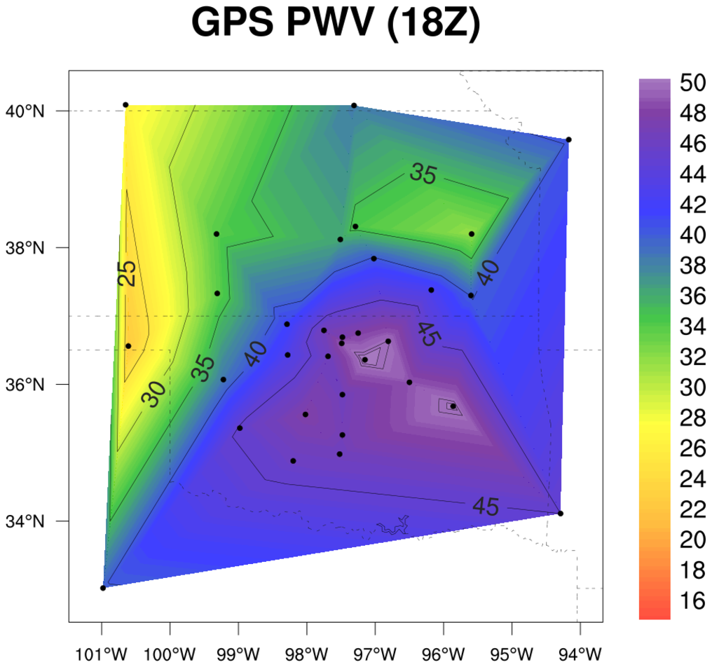
Import packages:
import numpy as np
import pandas as pd
import cartopy.crs as ccrs
import cartopy.feature as cfeature
from matplotlib import pyplot as plt

import geocat.datafiles as gdf
import geocat.viz as gv
Generate data:
# Open a ascii data file using pandas' read_csv function
ds = pd.read_csv(gdf.get('ascii_files/pw.dat'), delimiter='\\s+')

# Extract columns
pwv = ds.PW
pwv_lat1d = ds.LAT
pwv_lon1d = ds.LON
Plot
# Generate figure (set its size (width, height) in inches)
fig = plt.figure(figsize=(12, 10))

# Generate axes
ax = plt.axes(projection=ccrs.PlateCarree())

# Specify contour and contourf levels
clevels = np.arange(25, 51, 5)
flevels = np.arange(16, 51, 1)

# Plot contour lines
contour = ax.tricontour(
    pwv_lon1d, pwv_lat1d, pwv, levels=clevels, colors='black', linewidths=0.6, zorder=4
)

# Label the contours and set axes title
ax.clabel(contour, clevels, fontsize=25, fmt="%.0f")

# Plot filled contours
color = ax.tricontourf(
    pwv_lon1d,
    pwv_lat1d,
    pwv,
    cmap='magma',
    alpha=0.85,
    levels=flevels,
    antialiased=True,
    zorder=3,
)

# Add coordinate markers on the plot
ax.plot(pwv_lon1d, pwv_lat1d, marker='o', linewidth=0, color='black', zorder=4)

# Add state boundaries other lake features
ax.add_feature(cfeature.STATES, edgecolor='gray', linestyle=(0, (5, 10)), zorder=2)
ax.add_feature(cfeature.LAKES, facecolor='white', edgecolor='black', zorder=2)

# Use geocat.viz.util convenience function to set axes tick values
gv.set_axes_limits_and_ticks(
    ax,
    ylim=(min(pwv_lat1d) - 0.5, max(pwv_lat1d) + 0.5),
    xlim=(min(pwv_lon1d) - 0.5, max(pwv_lon1d) + 0.5),
    yticks=np.array([34, 36, 38, 40]),
    xticks=np.arange(-101, -93, 1),
)

# Use geocat.viz.util convenience function to set latitude, longitude tick labels
gv.add_lat_lon_ticklabels(ax)

# Use geocat.viz.util convenience function to add minor and major tick lines
gv.add_major_minor_ticks(ax, x_minor_per_major=1, y_minor_per_major=1, labelsize=18)

# Manually turn off ticks on top and right spines
ax.tick_params(axis='x', top=False)
ax.tick_params(axis='y', right=False)

# Add title
ax.set_title('GPS PWV(18Z)', fontweight='bold', fontsize=35, y=1.05)

# Force the plot to be square by setting the aspect ratio to 1
ax.set_box_aspect(1)

# Call tight_layout before adding colorbar to prevent user warning
plt.tight_layout()

# Set color bar axes
cax = fig.add_axes([0.9, 0.065, 0.04, 0.83])

# Add colorbar
cab = plt.colorbar(color, cax=cax, ticks=flevels[::2], drawedges=False, extendrect=True)

# Set colorbar ticklabel font size
cab.ax.yaxis.set_tick_params(length=0, labelsize=20)

# Show the plot
plt.show()
Ignoring fixed y limits to fulfill fixed data aspect with adjustable data limits.
Total running time of the script: (0 minutes 1.753 seconds)