NCL_mask_2.py

This script illustrates the following concepts:

• Using keyword zorder to mask areas in a plot

• Drawing filled land areas on top of a contour plot

• Selecting a different colormap to abide by best practices. See the color examples for more information.

See following URLs to see the reproduced NCL plot & script:

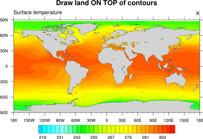
• Original NCL script: https://www.ncl.ucar.edu/Applications/Scripts/mask_2.ncl

• Original NCL plot: https://www.ncl.ucar.edu/Applications/Images/mask_2_lg.png

Using zorder:

The zorder keyword is used by matplotlib to layer elements in a plot. Elements with lower zorder values are plotted first and other elements are layered on top based on increasing zorder values. For more information, please refer to matplotlib’s zorder demo page.

Import packages:

import cartopy.crs as ccrs
import cartopy.feature as cfeature
from cartopy.mpl.gridliner import LongitudeFormatter, LatitudeFormatter
import matplotlib.pyplot as plt
import numpy as np
import xarray as xr

import geocat.datafiles as gdf
import geocat.viz as gv

Read in data:

# Open a netCDF data file using xarray and load the data into xarrays
# Disable time decoding due to missing necessary metadata
ds = xr.open_dataset(gdf.get("netcdf_files/atmos.nc"), decode_times=False)

# Extract a slice of the data at first time step
ds = ds.isel(time=0).drop("time")
TS = ds.TS

# Fix the artifact of not-shown-data around 0 and 360-degree longitudes
TS = gv.xr_add_cyclic_longitudes(TS, "lon")

Plot:

# Generate figure (set its size (width, height) in inches)
fig = plt.figure(figsize=(10, 6))

# Generate axes using Cartopy and draw land masses, coastlines, and lakes
ax = plt.axes(projection=ccrs.PlateCarree())
ax.add_feature(cfeature.LAND, facecolor='lightgray', zorder=1)
ax.add_feature(cfeature.COASTLINE, linewidth=0.5, zorder=1)
ax.add_feature(cfeature.LAKES,
               linewidth=0.5,
               edgecolor='black',
               facecolor='None',
               zorder=1)

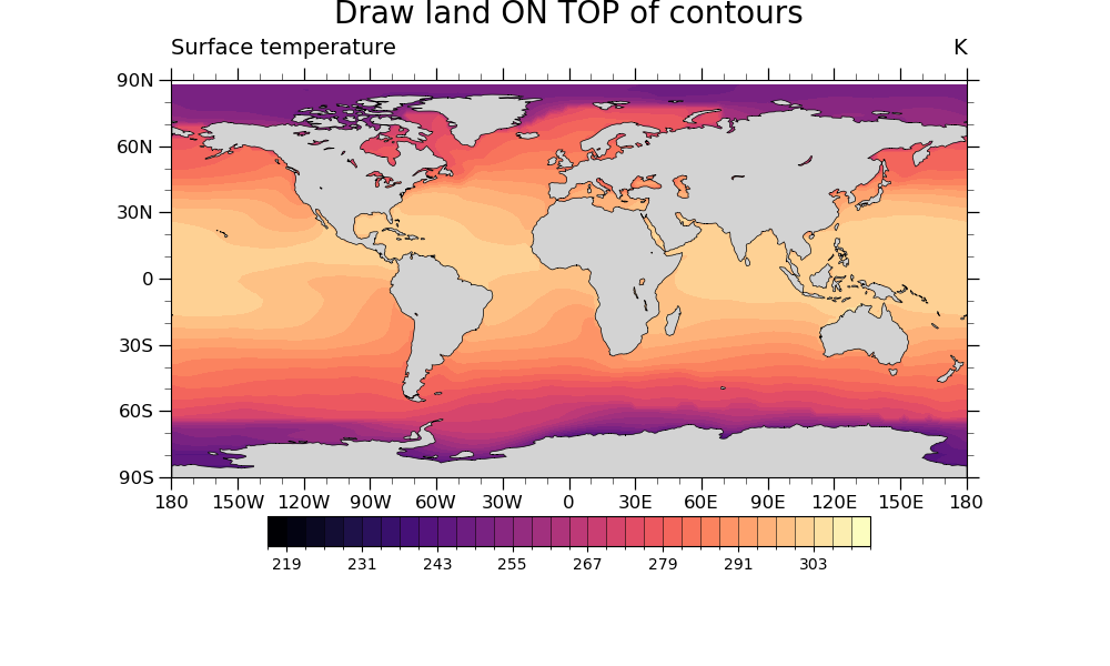
# Plot filled contour
contour = TS.plot.contourf(ax=ax,
                           transform=ccrs.PlateCarree(),
                           cmap='magma',
                           levels=np.arange(216, 315, 3),
                           extend='neither',
                           add_colorbar=False,
                           add_labels=False,
                           zorder=0)
plt.colorbar(contour,
             ax=ax,
             ticks=np.linspace(219, 303, 8),
             orientation='horizontal',
             pad=0.075,
             drawedges=True,
             shrink=0.7)

# Use geocat.viz.util convenience function to set axes limits & tick values
gv.set_axes_limits_and_ticks(ax,
                             xlim=(-180, 180),
                             ylim=(-90, 90),
                             xticks=np.linspace(-180, 180, 13),
                             yticks=np.linspace(-90, 90, 7))

# Use geocat.viz.util convenience function to add minor and major tick lines
gv.add_major_minor_ticks(ax, labelsize=12)

# Use geocat.viz.util convenience function to make latitude and
# longitude tick labels
gv.add_lat_lon_ticklabels(ax)
# Remove the degree symbol from tick labels
ax.yaxis.set_major_formatter(LatitudeFormatter(degree_symbol=''))
ax.xaxis.set_major_formatter(LongitudeFormatter(degree_symbol=''))

# Use geocat.viz.util convenience function to add titles
gv.set_titles_and_labels(ax,
                         maintitle='Draw land ON TOP of contours',
                         lefttitle=TS.long_name,
                         righttitle=TS.units,
                         lefttitlefontsize=14,
                         righttitlefontsize=14)

plt.show()