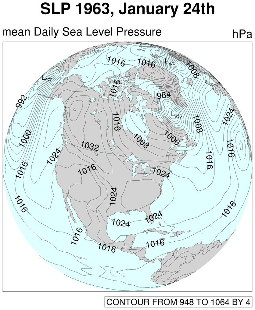
NCL_sat_1.py

This script illustrates the following concepts:

• Creating an orthographic projection

• Drawing line contours over a satellite map

• Manually labeling contours

• Transforming coordinates

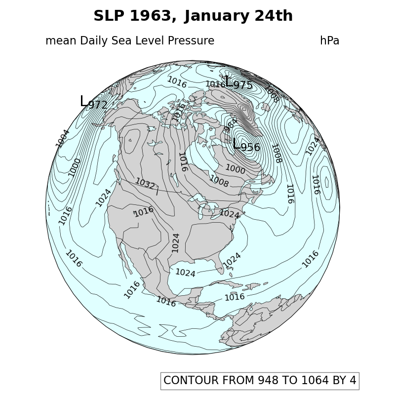
See following URLs to see the reproduced NCL plot & script:

• Original NCL script: https://www.ncl.ucar.edu/Applications/Scripts/sat_1.ncl

• Original NCL plot: https://www.ncl.ucar.edu/Applications/Images/sat_1_lg.png

Import packages:

import xarray as xr
import matplotlib.pyplot as plt
import cartopy.crs as ccrs
import cartopy.feature as cfeature
import numpy as np

import geocat.datafiles as gdf
import geocat.viz as gv

Read in data:

# Open a netCDF data file using xarray default engine and
# load the data into xarrays
ds = xr.open_dataset(gdf.get("netcdf_files/slp.1963.nc"), decode_times=False)

# Get data from the 24th timestep
pressure = ds.slp[24, :, :]

# Translate short values to float values
pressure = pressure.astype('float64')

# Convert Pa to hPa data
pressure = pressure * 0.01

# Fix the artifact of not-shown-data around 0 and 360-degree longitudes
wrap_pressure = gv.xr_add_cyclic_longitudes(pressure, "lon")

/home/docs/checkouts/readthedocs.org/user_builds/geocat-examples/conda/latest/lib/python3.11/site-packages/xarray/coding/times.py:170: SerializationWarning: Ambiguous reference date string: 1-1-1 00:00:0.0. The first value is assumed to be the year hence will be padded with zeros to remove the ambiguity (the padded reference date string is: 0001-1-1 00:00:0.0). To remove this message, remove the ambiguity by padding your reference date strings with zeros.
  warnings.warn(warning_msg, SerializationWarning)

Create plot

# Set figure size
fig = plt.figure(figsize=(8, 8))

# Set global axes with an orthographic projection
proj = ccrs.Orthographic(central_longitude=270, central_latitude=45)
ax = plt.axes(projection=proj)
ax.set_global()

# Add land, coastlines, and ocean features
ax.add_feature(cfeature.LAND, facecolor='lightgray')
ax.add_feature(cfeature.COASTLINE, linewidth=.5)
ax.add_feature(cfeature.OCEAN, facecolor='lightcyan')
ax.add_feature(cfeature.BORDERS, linewidth=.5)
ax.add_feature(cfeature.LAKES,
               facecolor='lightcyan',
               edgecolor='black',
               linewidth=.5)

# Make array of the contour levels that will be plotted
contours = np.arange(948, 1072, 4)

# Plot contour data
p = wrap_pressure.plot.contour(ax=ax,
                               transform=ccrs.PlateCarree(),
                               linewidths=0.5,
                               levels=contours,
                               cmap='black',
                               add_labels=False)

# regular pressure contour levels- These values were found by setting
# 'manual' argument in ax.clabel call to 'True' and then hovering mouse
# over desired location of countour label to find coordinate
# (which can be found in bottom left of figure window).
regularCLabels = [(176.4, 34.63), (-150.46, 42.44), (-142.16, 28.5),
                  (-134.12, 16.32), (-108.9, 17.08), (-98.17, 15.6),
                  (-108.73, 42.19), (-111.25, 49.66), (-127.83, 41.93),
                  (-92.49, 25.64), (-77.29, 29.08), (-77.04, 16.42),
                  (-95.93, 57.59), (-156.05, 84.47), (-17.83, 82.52),
                  (-76.3, 41.99), (-48.89, 41.45), (-33.43, 37.55),
                  (-46.98, 17.17), (1.79, 63.67), (-58.78, 67.05),
                  (-44.78, 53.68), (-69.69, 53.71), (-78.02, 52.22),
                  (-16.91, 44.33), (-95.72, 35.17), (-102.69, 73.62)]

# low pressure contour levels- these will be plotted
# as a subscript to an 'L' symbol.
lowCLabels = gv.find_local_extrema(pressure,
                                   eType='Low',
                                   highVal=1040,
                                   lowVal=975)

# Plot Clabels
gv.plot_contour_labels(ax,
                       p,
                       ccrs.Geodetic(),
                       proj,
                       clabel_locations=regularCLabels)
gv.plot_extrema_labels(pressure,
                       ccrs.Geodetic(),
                       proj,
                       label_locations=lowCLabels)

# Use gv function to set title and subtitles
gv.set_titles_and_labels(ax,
                         maintitle=r"$\bf{SLP}$" + " " + r"$\bf{1963,}$" + " " +
                         r"$\bf{January}$" + " " + r"$\bf{24th}$",
                         maintitlefontsize=20,
                         lefttitle="mean Daily Sea Level Pressure",
                         lefttitlefontsize=16,
                         righttitle="hPa",
                         righttitlefontsize=16)

# Set characteristics of text box
props = dict(facecolor='white', edgecolor='black', alpha=0.5)

# Place text box
ax.text(0.40,
        -0.1,
        'CONTOUR FROM 948 TO 1064 BY 4',
        transform=ax.transAxes,
        fontsize=16,
        bbox=props)

# Make layout tight
plt.tight_layout()

plt.show()

/home/docs/checkouts/readthedocs.org/user_builds/geocat-examples/checkouts/latest/Gallery/MapProjections/NCL_sat_1.py:104: UserWarning: The following locations could not be translated into the desired projection: (60.0, -60.0), (327.5, -60.0), (10.0, -62.5), (182.5, -62.5). These locations will be dropped.
  gv.plot_extrema_labels(pressure,