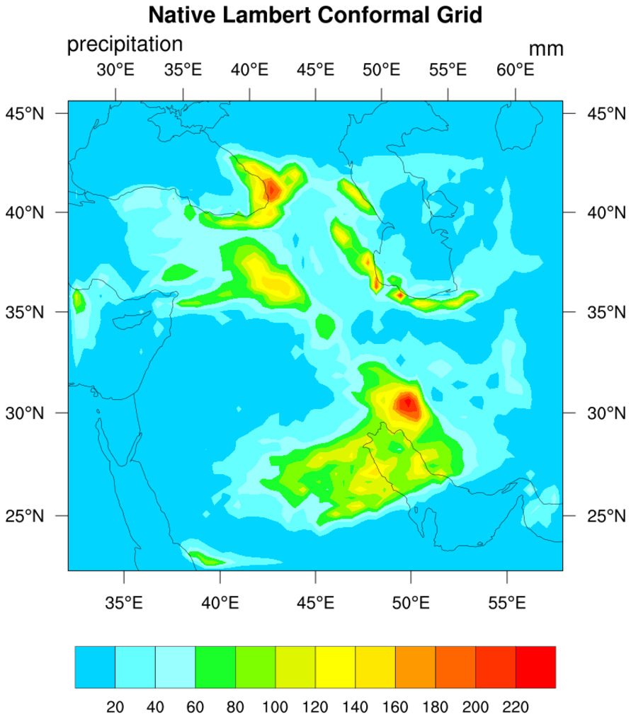
NCL_lcnative_1.py

This script illustrates the following concepts:

• Drawing contours over a map using a native lat,lon grid

• Drawing filled contours over a Lambert Conformal map

• Zooming in on a particular area on a Lambert Conformal map

• Subsetting a color map

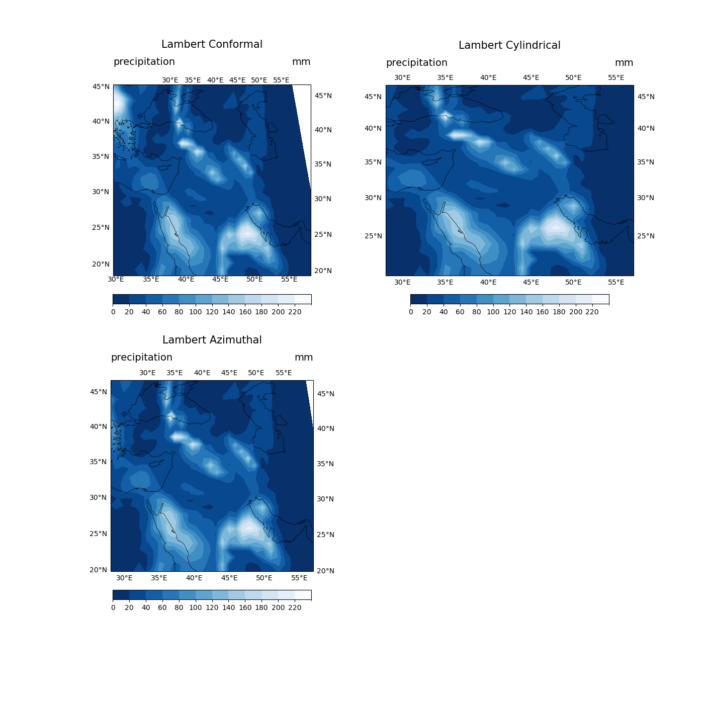
• Using all three Cartopy Lambert projections to find the best fit for visualization

• Implementing best practices for choosing contour color scheme. The original NCL version uses a rainbow color map which can create problems for individuals impacted by color blindness and is not black and white printer friendly. To overcome this, we used the “Blues_r” color scheme from Matplotlib. More information on best practices can be found here.

See following URLs to see the reproduced NCL plot & script:

• Original NCL script: https://www.ncl.ucar.edu/Applications/Scripts/lcnative_1.ncl

• Original NCL plot: https://www.ncl.ucar.edu/Applications/Images/lcnative_1_lg.png

Import packages:

import numpy as np
import xarray as xr
import cartopy.crs as ccrs
import matplotlib.pyplot as plt
import matplotlib.ticker as mticker

import geocat.datafiles as gdf

Read in data:

# Open a netCDF data file using xarray default engine and load the data into xarrays
ds = xr.open_dataset(gdf.get("netcdf_files/pre.8912.mon.nc"),
                     decode_times=False)

# Extract a slice of the data
t = ds.pre.isel(time=0)

Plot:

plt.figure(figsize=(14, 14))


def Plot(row, col, pos, proj, title):
    '''
    Args:

        row (:class: 'int'):
            number of rows necessary for subplotting of visualizations
        col (:class: 'int'):
            number of columns necessary for subplotting
        pos (:class: 'int'):
            position of visualization in m x n subplot
        proj (:class: 'cartopy.crs'):
            which projection to visualize
        title (:class: 'str'):
            center title of respective visualization
    '''
    # Generate axes using Cartopy and draw coastlines
    ax = plt.subplot(row, col, pos, projection=proj)
    ax.set_extent((28, 57, 20, 47), crs=ccrs.PlateCarree())
    ax.coastlines(linewidth=0.5)

    # Use ax "gridlines" function to draw lat/lon markers on projections
    gl = ax.gridlines(draw_labels=True,
                      dms=False,
                      x_inline=False,
                      y_inline=False)
    gl.top_labels = True
    gl.right_labels = True
    gl.xlines = False
    gl.ylines = False
    gl.xlocator = mticker.FixedLocator([30, 35, 40, 45, 50, 55])
    gl.ylocator = mticker.FixedLocator([20, 25, 30, 35, 40, 45])
    gl.xlabel_style = {'rotation': 0}
    gl.ylabel_style = {'rotation': 0}
    '''
    When using certain types of projections in Cartopy, you may find that there
    is not a direct 1-to-1 projection similarity. When looking at the three Lambert
    projections offered, you will notice the closest match to the NCL projection
    is actually the Lambert Cylindrical projection. This is due to NCL having certain
    "smoothing" and "flattening" options for the Lambert Conformal projection not seen
    in the Cartopy version. By using Lambert Cylindrical over Lambert Conformal in Python,
    you will be able to create the "rectangular" style of coordinates not classically
    represented by a Lambert Conformal map. Additionally, Cartopy does not currently support
    adding tick marks to a projection like NCL, this is why these Python projections do not
    have this feature. The GeoCAT Team is actively adding to the list of convenience functions
    supported and hopes to add this functionality one day.
    '''

    # Plot data and create colorbar
    prec = t.plot.contourf(ax=ax,
                           cmap="Blues_r",
                           transform=ccrs.PlateCarree(),
                           levels=14,
                           add_colorbar=False)

    cbar_ticks = np.arange(0, 240, 20)
    cbar = plt.colorbar(prec,
                        orientation='horizontal',
                        pad=0.075,
                        shrink=0.8,
                        ticks=cbar_ticks)

    cbar.ax.tick_params(labelsize=10)
    plt.title(title, loc='center', y=1.17, size=15)
    plt.title(t.units, loc='right', y=1.08, size=14)
    plt.title("precipitation", loc='left', y=1.08, size=14)


Plot(
    2, 2, 1,
    ccrs.LambertConformal(central_longitude=45,
                          standard_parallels=(36, 55),
                          globe=ccrs.Globe()), "Lambert Conformal")
Plot(2, 2, 2, ccrs.LambertCylindrical(central_longitude=45),
     "Lambert Cylindrical")
Plot(2, 2, 3, ccrs.LambertAzimuthalEqualArea(central_longitude=45),
     "Lambert Azimuthal")