

Note
Go to the end to download the full example code.
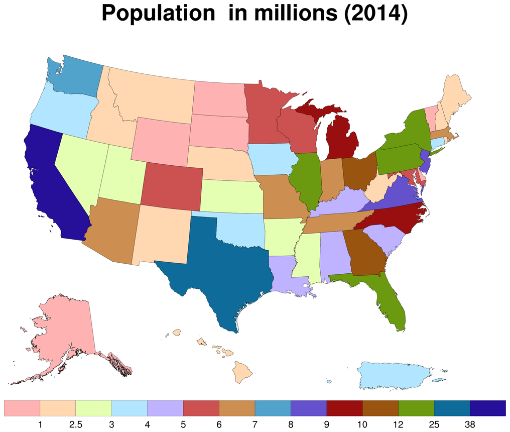
NCL_polyg_19.py#
- This script illustrates the following concepts:
Adding lines and polygons to a map
Adding a map to another map as an annotation
Coloring shapefile outlines based on an array of values
Drawing a custom colorbar on a map
Using functions for cleaner code
Overlaying a shape from one shapefile over another
- See following URLs to see the reproduced NCL plot & script:
Original NCL script: https://www.ncl.ucar.edu/Applications/Scripts/polyg_19.ncl
Original NCL plot: https://www.ncl.ucar.edu/Applications/Images/polyg_19_lg.png
Import packages:
import matplotlib.pyplot as plt
import matplotlib.gridspec as gridspec
from matplotlib.collections import PatchCollection
from matplotlib.patches import Polygon
import matplotlib.colors as colors
from mpl_toolkits.axes_grid1.inset_locator import inset_axes
import matplotlib.cm as cm
import shapefile as shp
import numpy as np

import geocat.datafiles as gdf
import geocat.viz as gv
Read in data:
# Open all shapefiles and associated .dbf, .shp, and .prj files so sphinx can run and generate documents
file1 = open(gdf.get("shape_files/gadm36_USA_1.dbf"), 'r')
file2 = open(gdf.get("shape_files/gadm36_USA_1.shp"), 'r')
file3 = open(gdf.get("shape_files/gadm36_USA_1.shx"), 'r')
file4 = open(gdf.get("shape_files/gadm36_USA_1.prj"), 'r')

file5 = open(gdf.get("shape_files/gadm36_USA_2.dbf"), 'r')
file6 = open(gdf.get("shape_files/gadm36_USA_2.shp"), 'r')
file7 = open(gdf.get("shape_files/gadm36_USA_2.shx"), 'r')
file8 = open(gdf.get("shape_files/gadm36_USA_2.prj"), 'r')

file9 = open(gdf.get("shape_files/gadm36_PRI_0.dbf"), 'r')
file10 = open(gdf.get("shape_files/gadm36_PRI_0.shp"), 'r')
file11 = open(gdf.get("shape_files/gadm36_PRI_0.shx"), 'r')
file12 = open(gdf.get("shape_files/gadm36_PRI_0.prj"), 'r')

# Open the text file with the population data
state_population_file = open(gdf.get("ascii_files/us_state_population.txt"), 'r')
# Open shapefiles
us = shp.Reader(gdf.get("shape_files/gadm36_USA_1.dbf"))
usdetailed = shp.Reader(gdf.get("shape_files/gadm36_USA_2.dbf"))
pr = shp.Reader(gdf.get("shape_files/gadm36_PRI_0.dbf"))
Set colormap data and colormap bounds:
colormap = colors.ListedColormap(
    [
        'lightpink',
        'wheat',
        'palegreen',
        'powderblue',
        'thistle',
        'lightcoral',
        'peru',
        'dodgerblue',
        'slateblue',
        'firebrick',
        'sienna',
        'olivedrab',
        'steelblue',
        'navy',
    ]
)

colorbounds = [0, 1, 2.5, 3, 4, 5, 6, 7, 8, 9, 10, 12, 25, 38, 40]

norm = colors.BoundaryNorm(colorbounds, colormap.N)
Define helper function to get the populations of each state
def getStatePopulations(state_population_file):
    population_dict = {}
    Lines = state_population_file.read().splitlines()
    for line in Lines:
        nameandpop = line.split(" ")
        if nameandpop[-1].isnumeric():
            name = nameandpop[0]
            pop = (int)(nameandpop[-1]) / 1000000
            population_dict[name] = pop
    return population_dict
Define helper function to get the color of each state based on its population
def findDivColor(colorbounds, pdata):
    for x in range(len(colorbounds)):
        if pdata >= colorbounds[len(colorbounds) - 1]:
            return colormap.colors[x - 1]
        if pdata >= colorbounds[x]:
            continue
        else:
            # Index is 'x-1' because colorbounds is one item longer than colormap
            return colormap.colors[x - 1]
Define helper function to remove ticks from axes
def removeTicks(axis):
    axis.get_xaxis().set_visible(False)
    axis.get_yaxis().set_visible(False)
Define helper function to plot and color each state
def plotRegion(region, axis, xlim, puertoRico, waterBody):
    # Create empty lists for filled polygons or" patches" and "water_patches"
    patches = []
    water_patches = []

    # Plot each shape within a region (ex. mainland Alaska and all of it's surrounding Alaskan islands)
    for i in range(len(region.shape.parts)):
        i_start = region.shape.parts[i]
        if i == len(region.shape.parts) - 1:
            i_end = len(region.shape.points)
        else:
            i_end = region.shape.parts[i + 1]

        # Create new empty lists to hold lat and lon coordinates
        x = []
        y = []

        # Get every coordinate within every shape (as long as it is within the x coordinate limits)
        for i in region.shape.points[i_start:i_end]:
            if xlim[0] is not None and i[0] < xlim[0]:
                continue
            if xlim[1] is not None and i[0] > xlim[1]:
                continue
            else:
                x.append(i[0])
                y.append(i[1])

        # Plot outline of each region
        axis.plot(x, y, color='black', linewidth=0.1, zorder=1)

        # Fill each state with color:
        # Determine the region to be plotted (Puerto Rico or United States)
        if waterBody is False:
            if puertoRico is False:
                abbrevname = shape.record[-1].split(".")
                abbrevstate = abbrevname[1]
            else:
                abbrevstate = 'PR'

        # If the region being plotted is a state with a population
        if waterBody is False:
            pop = population_dict[abbrevstate]
            color = findDivColor(colorbounds, pop)
            # Set characteristics and measurements of each filled polygon "patch"
            patches.append(
                Polygon(np.vstack((x, y)).T, closed=True, color=color, linewidth=0.1)
            )

        # If the region being plotted is a body of water with no population
        else:
            # Set characteristics and measurements of each filled polygon "patch"
            water_patches.append(
                Polygon(np.vstack((x, y)).T, closed=True, color='white', linewidth=0.7)
            )

    pc = PatchCollection(
        patches, match_original=True, edgecolor='k', linewidths=0.1, zorder=2
    )
    # Plot filled region on axis
    axis.add_collection(pc)

    wpc = PatchCollection(
        water_patches, match_original=True, edgecolor='white', linewidth=0.8, zorder=3
    )
    # Plot filled region on axis
    axis.add_collection(wpc)
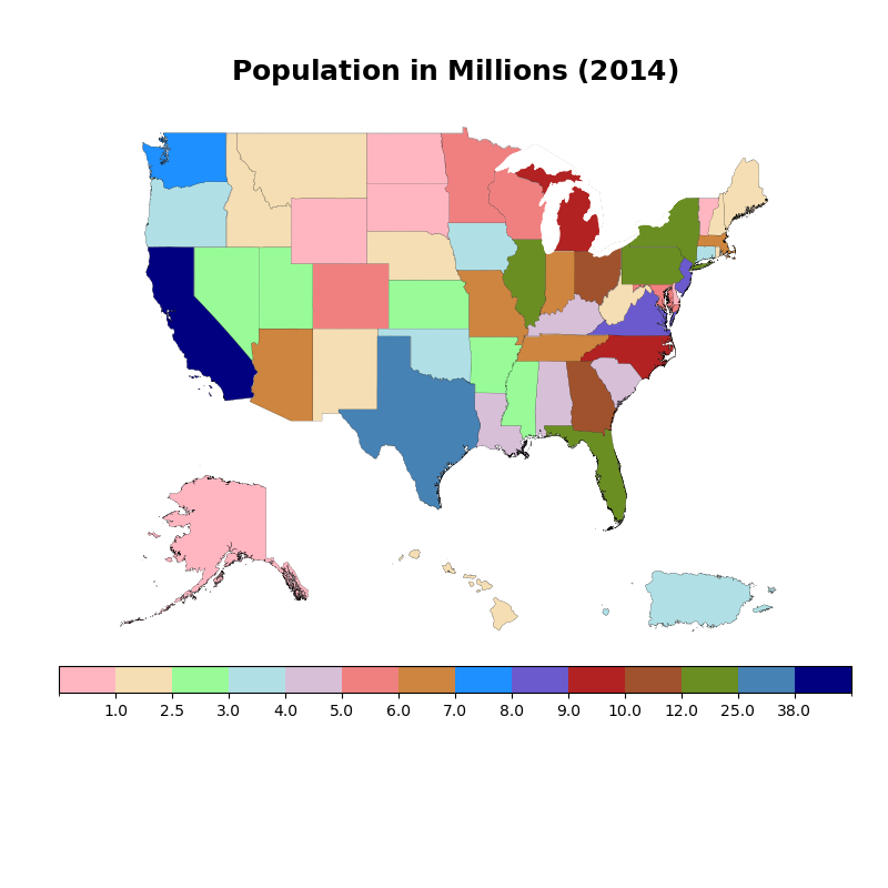
Plot:
# Create figure
fig = plt.figure(figsize=(8, 8))
spec = gridspec.GridSpec(
    ncols=1, nrows=2, hspace=0.05, wspace=0.1, figure=fig, height_ratios=[2, 1]
)

# Create upper axis
ax1 = fig.add_subplot(spec[0, 0], frameon=False)
removeTicks(ax1)

# Create lower axis
ax2 = fig.add_subplot(spec[1, 0], frameon=False)
removeTicks(ax2)

# Create three inset axes on lower axis for Alaska, Hawaii, and Puerto Rico respectively
axin1 = ax2.inset_axes([0.0, 0.7, 0.30, 0.80], frameon=False)
removeTicks(axin1)
axin2 = ax2.inset_axes([0.40, 0.7, 0.20, 0.40], frameon=False)
removeTicks(axin2)
axin3 = ax2.inset_axes([0.70, 0.7, 0.30, 0.30], frameon=False)
removeTicks(axin3)

# Get population of each state
population_dict = getStatePopulations(state_population_file)

# Plot every shape in the US shapefile
for shape in us.shapeRecords():
    if shape.record[3] == 'Alaska':
        plotRegion(shape, axin1, [None, 100], puertoRico=False, waterBody=False)
    elif shape.record[3] == 'Hawaii':
        plotRegion(shape, axin2, [-161, None], puertoRico=False, waterBody=False)
    else:
        plotRegion(shape, ax1, [None, None], puertoRico=False, waterBody=False)

# Plot every shape in the puerto rico shapefile
for shape in pr.shapeRecords():
    plotRegion(shape, axin3, [None, None], puertoRico=True, waterBody=False)

# Plot every body of water shape in the detailed US shapefile
for shape in usdetailed.shapeRecords():
    if shape.record[9] == 'Water body':
        plotRegion(shape, ax1, [None, None], puertoRico=False, waterBody=True)

# Set title using helper function from geocat-viz
title = (
    r"$\bf{Population}$"
    + " "
    + r"$\bf{in}$"
    + " "
    + r"$\bf{Millions}$"
    + " "
    + r"$\bf{(2014)}$"
)
gv.set_titles_and_labels(ax1, maintitle=title, maintitlefontsize=18)

# Create fourth inset axis for colorbar
axin4 = inset_axes(ax2, width="115%", height="12%", loc='center')

# Create colorbar
cb = fig.colorbar(
    cm.ScalarMappable(cmap=colormap, norm=norm),
    cax=axin4,
    boundaries=colorbounds,
    ticks=colorbounds[1:-1],
    spacing='uniform',
    orientation='horizontal',
)

plt.show()
Total running time of the script: (0 minutes 14.228 seconds)