NCL_skewt_1.py

This script illustrates the following concepts:

• Drawing a default Skew-T background

• Customizing the background of a Skew-T plot

See following URLs to see the reproduced NCL plot & script:

• Original NCL script: https://www.ncl.ucar.edu/Applications/Scripts/skewt_1.ncl

• Original NCL plots: https://www.ncl.ucar.edu/Applications/Images/skewt_1_1_lg.png and https://www.ncl.ucar.edu/Applications/Images/skewt_1_2_lg.png and https://www.ncl.ucar.edu/Applications/Images/skewt_1_3_lg.png

Import packages:

import matplotlib.pyplot as plt
import matplotlib.lines as mlines
import numpy as np
from metpy.plots import SkewT
from metpy.units import units

import geocat.viz as gv

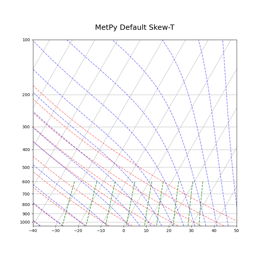
Plot Skew-T with MetPy Defaults:

# Note that there are no labels on the axes. This is because we have not yet
# plotted any data. Once data is plotted, MetPy will use the units of the
# data to create appropriate labels.
fig = plt.figure(figsize=(9, 9))
skew = SkewT(fig)
ax = skew.ax

skew.plot_dry_adiabats()
skew.plot_moist_adiabats()
skew.plot_mixing_lines()

gv.set_titles_and_labels(ax, maintitle="MetPy Default Skew-T")
plt.show()

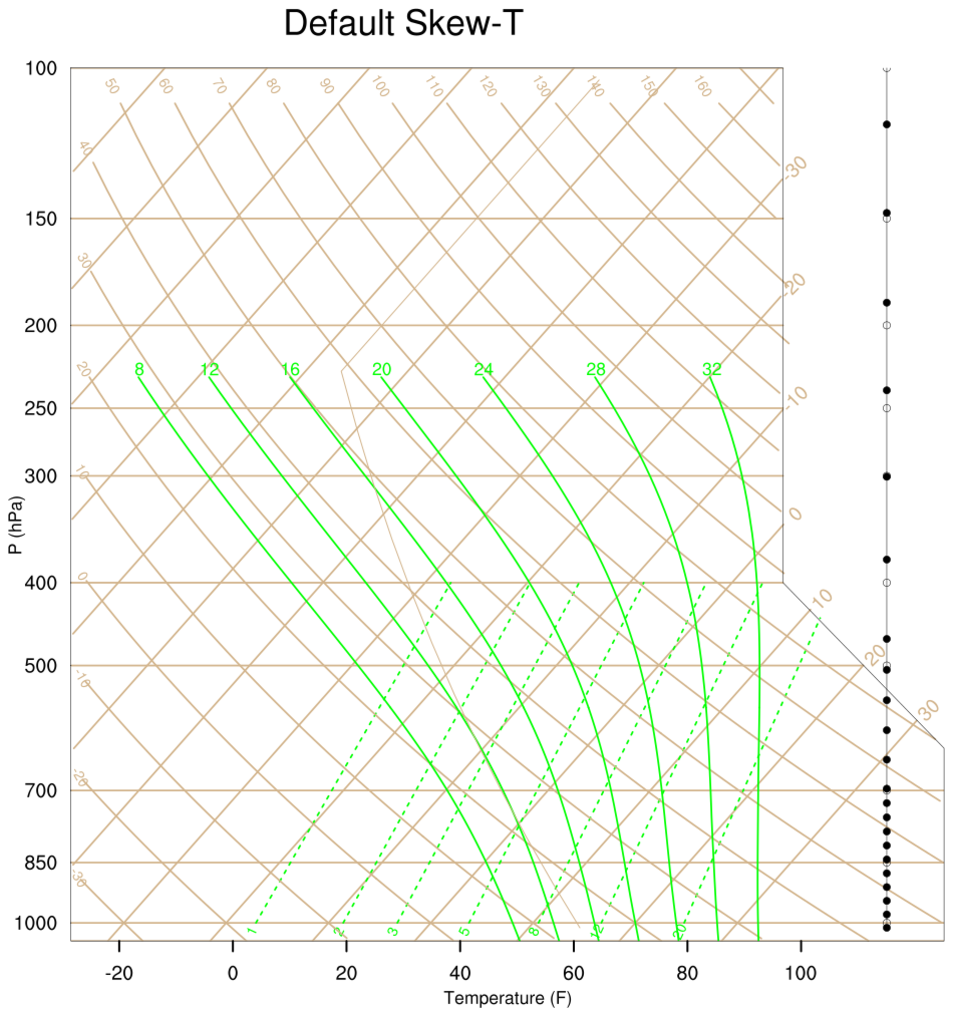
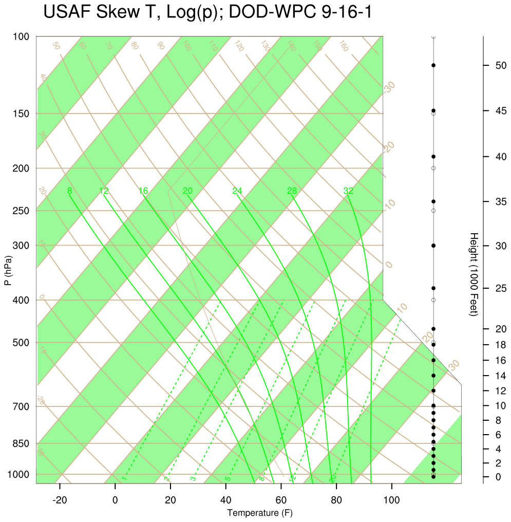
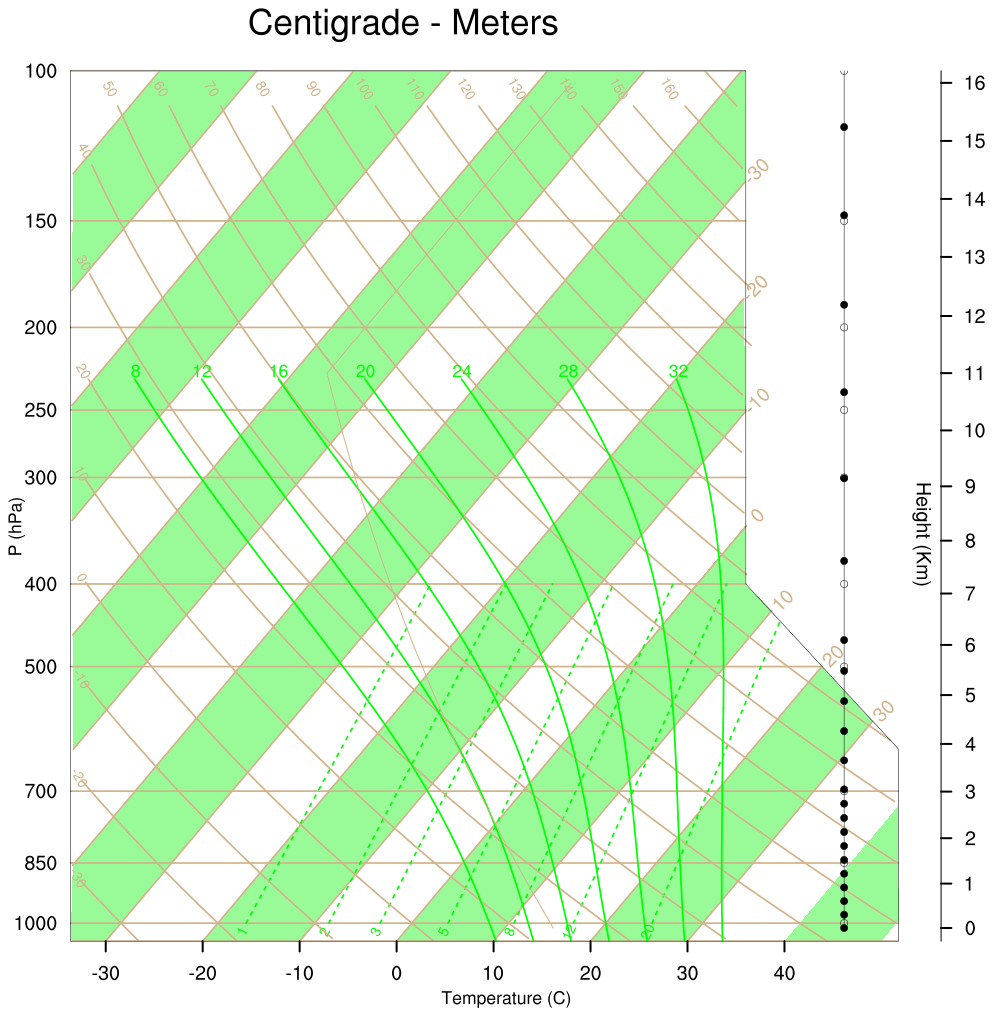
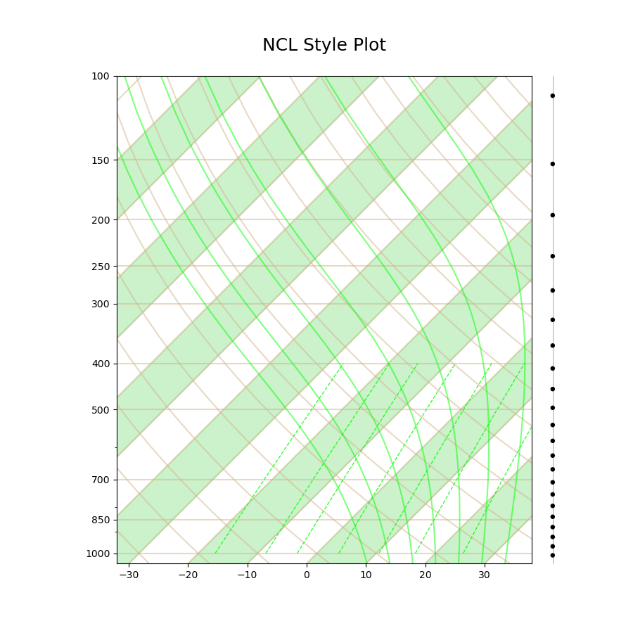
Plot Skew-T that is similar to NCL’s default Skew-T plot:

# Note that MetPy forces the x axis scale to be in Celsius and the y axis
# scale to be in hectoPascals. Once data is plotted, then the axes labels are
# automatically added
fig = plt.figure(figsize=(9, 9))

# The rotation keyword changes how skewed the temperature lines are. MetPy has
# a default skew of 30 degrees
skew = SkewT(fig, rotation=45)
ax = skew.ax

# Shade every other section between isotherms
x1 = np.linspace(-100, 40, 8)  # The starting x values for the shaded regions
x2 = np.linspace(-90, 50, 8)  # The ending x values for the shaded regions
y = [1050, 100]  # The range of y values that the shades regions should cover
for i in range(0, 8):
    skew.shade_area(y=y, x1=x1[i], x2=x2[i], color='limegreen', alpha=0.25, zorder=1)

# Choose starting temperatures in Kelvin for the dry adiabats
t0 = units.K * np.arange(243.15, 444.15, 10)
skew.plot_dry_adiabats(t0=t0, linestyles='solid', colors='tan', linewidths=1.5)

# Choose starting temperatures in Kelvin for the moist adiabats
t0 = units.K * np.arange(281.15, 306.15, 4)
skew.plot_moist_adiabats(t0=t0, linestyles='solid', colors='lime', linewidth=1.5)

# Choose mixing ratios
w = np.array([0.001, 0.002, 0.003, 0.005, 0.008, 0.012, 0.020]).reshape(-1, 1)

# Choose the range of pressures that the mixing ratio lines are drawn over
p = units.hPa * np.linspace(1000, 400, 7)

# Plot mixing ratio lines
skew.plot_mixing_lines(
    mixing_ratio=w, pressure=p, linestyle='dashed', colors='lime', linewidths=1
)

# Use geocat.viz utility functions to set axes limits and ticks
gv.set_axes_limits_and_ticks(
    ax=ax, xlim=[-32, 38], yticks=[1000, 850, 700, 500, 400, 300, 250, 200, 150, 100]
)

# Use geocat.viz utility functions to add a main title
gv.set_titles_and_labels(ax=ax, maintitle="NCL Style Plot")

# Plot empty wind barbs with dummy data
u = np.zeros(22)
v = u
p = np.linspace(1010, 110, 22)
skew.plot_barbs(
    pressure=p,
    u=u,
    v=v,
    xloc=1.05,
    fill_empty=True,
    sizes=dict(emptybarb=0.075, width=0.1, height=0.2),
)

# Draw line underneath wind barbs
line = mlines.Line2D(
    [1.05, 1.05],
    [0, 1],
    color='gray',
    linewidth=0.5,
    transform=ax.transAxes,
    clip_on=False,
    zorder=1,
)
ax.add_line(line)

# Change the style of the gridlines
plt.grid(True, which='major', axis='both', color='tan', linewidth=1.5, alpha=0.5)

plt.show()