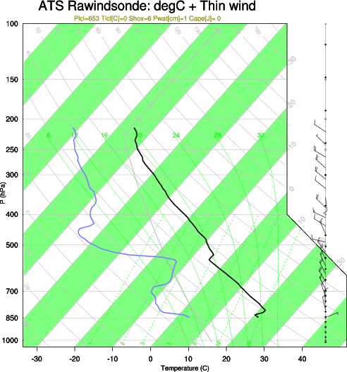
NCL_skewt_3_2.py

This script illustrates the following concepts:

• Drawing Skew-T plots

• Thinning the wind barbs in a Skew-T plot

• Customizing the background of a Skew_T plot

See following URLs to see the reproduced NCL plot & script:

• Original NCL script: https://www.ncl.ucar.edu/Applications/Scripts/skewt_3.ncl

• Original NCL plot: https://www.ncl.ucar.edu/Applications/Images/skewt_3_2_lg.png

Import packages:

import numpy as np
import matplotlib.pyplot as plt
import matplotlib.lines as mlines
import pandas as pd
import metpy.calc as mpcalc
from metpy.plots import SkewT
from metpy.units import units

import geocat.datafiles as gdf
import geocat.viz as gv

Read in data:

# Open a ascii data file using pandas' read_csv function
ds = pd.read_csv(gdf.get('ascii_files/sounding_ATS.csv'), header=None)

# Extract the data
p = ds[0].values  # Pressure [mb/hPa] (unitless for plot_barbs)
tc = ds[1].values * units.degC  # Temperature [C]
tdc = ds[2].values * units.degC  # Dew pt temp  [C]
wspd = ds[5].values * units.knots  # Wind speed   [knots or m/s]
wdir = ds[6].values * units.degrees  # Meteorological wind dir
u, v = mpcalc.wind_components(wspd, wdir)  # Calculate wind components

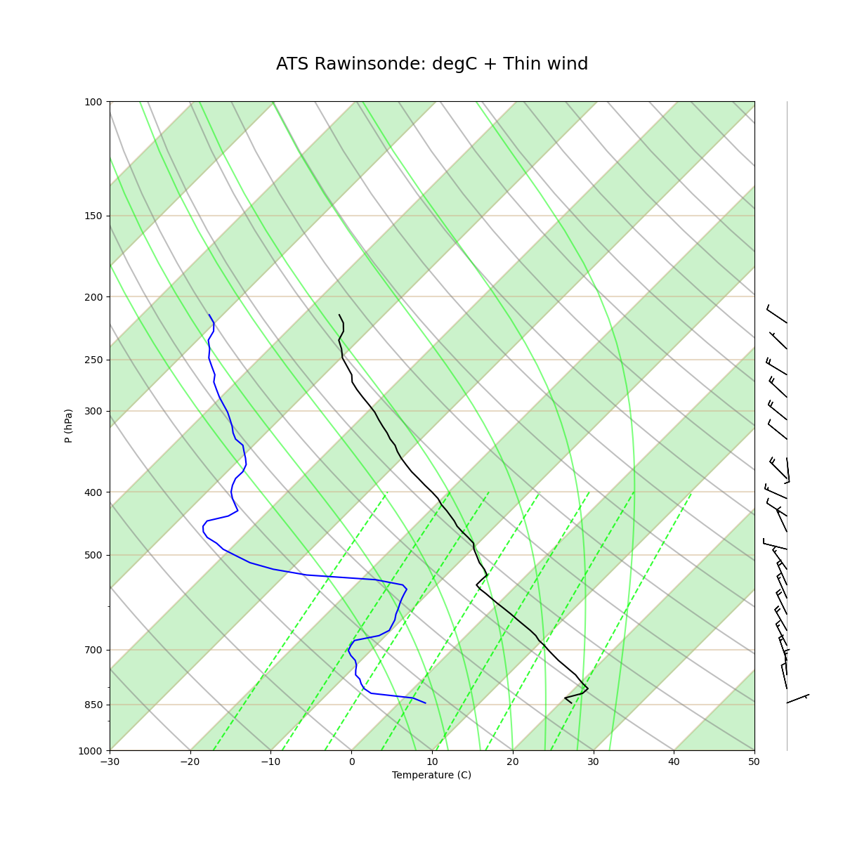
Plot

fig = plt.figure(figsize=(12, 12))

# Adding the "rotation" kwarg will over-ride the default MetPy rotation of
# 30 degrees for the 45 degree default found in NCL Skew-T plots
skew = SkewT(fig, rotation=45)
ax = skew.ax

# Shade every other section between isotherms
x1 = np.linspace(-100, 40, 8)  # The starting x values for the shaded regions
x2 = np.linspace(-90, 50, 8)  # The ending x values for the shaded regions
y = [1050, 100]  # The range of y values that the shaded regions should cover

for i in range(0, 8):
    skew.shade_area(y=y,
                    x1=x1[i],
                    x2=x2[i],
                    color='limegreen',
                    alpha=0.25,
                    zorder=1)

skew.plot(p, tc, 'black')
skew.plot(p, tdc, 'blue')
# Plot only every third windbarb
skew.plot_barbs(pressure=p[::3],
                u=u[::3],
                v=v[::3],
                xloc=1.05,
                fill_empty=True,
                sizes=dict(emptybarb=0.075, width=0.1, height=0.2))

# Draw line underneath wind barbs
line = mlines.Line2D([1.05, 1.05], [0, 1],
                     color='gray',
                     linewidth=0.5,
                     transform=ax.transAxes,
                     dash_joinstyle='round',
                     clip_on=False,
                     zorder=0)
ax.add_line(line)

# Add relevant special lines
# Choose starting temperatures in Kelvin for the dry adiabats
t0 = units.K * np.arange(243.15, 473.15, 10)
skew.plot_dry_adiabats(t0=t0, linestyles='solid', colors='gray', linewidth=1.5)

# Choose temperatures for moist adiabats
t0 = units.K * np.arange(281.15, 306.15, 4)
msa = skew.plot_moist_adiabats(t0=t0,
                               linestyles='solid',
                               colors='lime',
                               linewidths=1.5)

# Choose mixing ratios
w = np.array([0.001, 0.002, 0.003, 0.005, 0.008, 0.012, 0.020]).reshape(-1, 1)

# Choose the range of pressures that the mixing ratio lines are drawn over
p_levs = units.hPa * np.linspace(1000, 400, 7)
skew.plot_mixing_lines(mixing_ratio=w, pressure=p_levs, colors='lime')

skew.ax.set_ylim(1000, 100)

gv.set_titles_and_labels(ax, maintitle="ATS Rawinsonde: degC + Thin wind")

# Set axes limits and ticks
gv.set_axes_limits_and_ticks(
    ax=ax,
    xlim=[-30, 50],
    yticks=[1000, 850, 700, 500, 400, 300, 250, 200, 150, 100])

# Change the style of the gridlines
plt.grid(True,
         which='major',
         axis='both',
         color='tan',
         linewidth=1.5,
         alpha=0.5)
plt.xlabel("Temperature (C)")
plt.ylabel("P (hPa)")
plt.show()