

Note
Go to the end to download the full example code.
NCL_overlay_12.py#
- This script illustrates the following concepts:
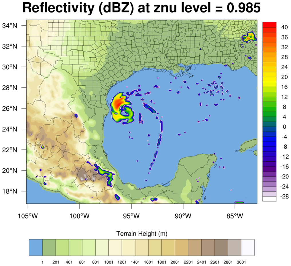
Overlaying WRF “dbz” on a topographic map
Using two different colormaps on one page
Drawing a custom color bar using matplotlib.cm.ScalarMappable
Using alpha argument to emphasize or subdue overlain features
Overlay multiple contours
Using shapefile data to plot United States county borders
Using zorder to specify the order in which elements will be drawn
Using inset_axes() to create additional axes for color bars
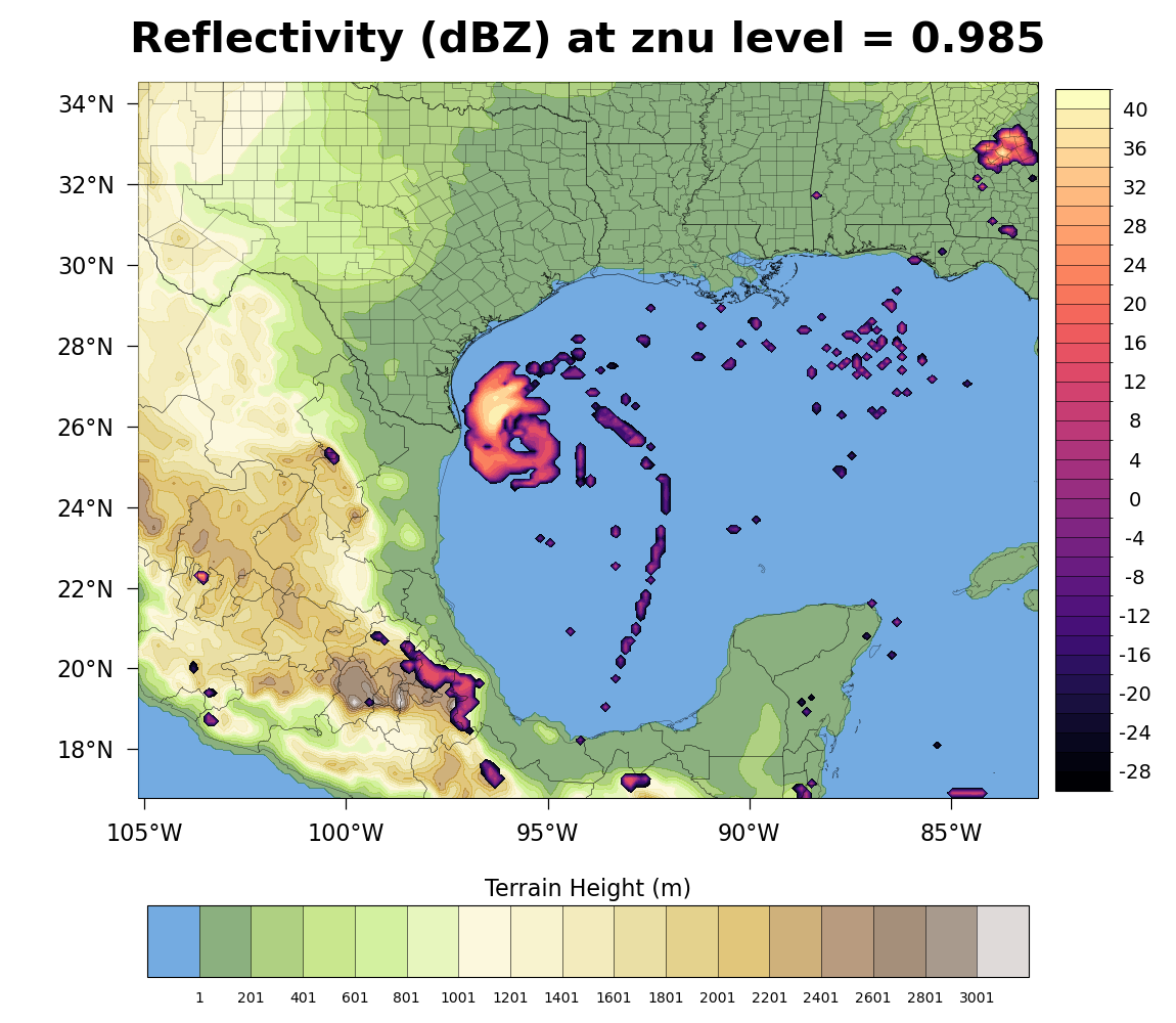
Using a different color scheme to follow best practices for visualizations
- See following URLs to see the reproduced NCL plot & script:
Original NCL script: https://www.ncl.ucar.edu/Applications/Scripts/overlay_12.ncl
Original NCL plots: https://www.ncl.ucar.edu/Applications/Images/overlay_12_1_lg.png
Import packages:
import numpy as np
from wrf import getvar
import cartopy.crs as ccrs
import cartopy.feature as cfeature
import cartopy.io.shapereader as shpreader
from netCDF4 import Dataset
import geocat.datafiles as gdf

import matplotlib.pyplot as plt
import matplotlib.cm as cm
import matplotlib.colors as mcolors
from mpl_toolkits.axes_grid1.inset_locator import inset_axes
import geocat.viz as gv
import cmaps
Read in data
# Read in the dataset
wrfin = Dataset(
    gdf.get("netcdf_files/wrfout_d01_2003-07-15_00_00_00"), decode_times=True
)

# Read variables
hgt = getvar(wrfin, "HGT")  # terrain height in m
lat = getvar(wrfin, "XLAT")  # latitude, south is negative
lon = getvar(wrfin, "XLONG")  # longitude, west is negative
znu = getvar(wrfin, "ZNU")  # eta values
dbz = getvar(wrfin, "dbz")[0, :, :]  # radar reflectivity in dBZ

# Open all shapefiles and associated .dbf, .shp, and .prj files
open(gdf.get("shape_files/countyl010g.dbf"), 'r')
open(gdf.get("shape_files/countyl010g.shp"), 'r')
open(gdf.get("shape_files/countyl010g.shx"), 'r')
open(gdf.get("shape_files/countyl010g.prj"), 'r')

# Open shapefiles
shapefile = shpreader.Reader(gdf.get("shape_files/countyl010g.dbf"))
Debug information
# This print output resembles NCL printMinMax function
print("------------------------------------------")
print(
    "{} ({}) : min={:.1f}    max={:.3f}".format(
        hgt.attrs['description'], hgt.attrs['units'], hgt.min().data, hgt.max().data
    )
)
print(
    "{} ({}) : min={:.1f}    max={:.3f}".format(
        dbz.attrs['description'], dbz.attrs['units'], dbz.min().data, dbz.max().data
    )
)
------------------------------------------
Terrain Height (m) : min=0.0    max=3213.484
radar reflectivity (dBZ) : min=-30.0    max=40.010
Create plot
# Generate figure (set its size (width, height) in inches)
fig = plt.figure(figsize=(11.5, 10))

# Get Cartopy projection
projection = ccrs.PlateCarree()

# Set axes [left, bottom, width, height] to leave space for color bars and titles
ax = plt.axes([0.05, 0.22, 0.9, 0.7], projection=projection)

# Create inset axes for color bars
cax1 = inset_axes(
    ax,
    width='98%',
    height='10%',
    loc='lower left',
    bbox_to_anchor=(0.01, -0.25, 1, 1),
    bbox_transform=ax.transAxes,
    borderpad=0,
)
cax2 = inset_axes(
    ax,
    width='6%',
    height='98%',
    loc='lower right',
    bbox_to_anchor=(0.08, 0.01, 1, 1),
    bbox_transform=ax.transAxes,
    borderpad=0,
)

# Set latitude and longitude extent to zoom in on map
ax.set_extent(
    [lon.min().data, lon.max().data, lat.min().data, lat.max().data], projection
)

#
# Add state and county borders
#

# Add US states borders
ax.add_feature(
    cfeature.NaturalEarthFeature(
        category='cultural',
        name='admin_1_states_provinces',
        scale='10m',
        facecolor='none',
        edgecolor='black',
        linewidth=0.2,
        zorder=5,
    )
)

# Add US county borders
counties = list(shapefile.geometries())
COUNTIES = cfeature.ShapelyFeature(counties, ccrs.PlateCarree())
ax.add_feature(COUNTIES, facecolor='none', edgecolor='black', linewidth=0.2, zorder=5)

#
# Plot terrain height contour
#

# Import NCL color map
cmap = cmaps.OceanLakeLandSnow

# Set contour levels
levels = np.array([0, 1] + [i for i in range(201, 3202, 200)])

# Contourf hgt data
contour = ax.contourf(lon, lat, hgt.data, alpha=0.6, levels=levels, cmap=cmap, zorder=3)
# Add first color bar
clb = fig.colorbar(
    contour, cax=cax1, orientation='horizontal', ticks=levels[1:-1], drawedges=True
)

# Manually set color bar tick length and tick labels padding.
clb.ax.xaxis.set_tick_params(length=0, pad=10)

# Set color bar label and fontsize. labelpad controls the vertical location relative to the color bar.
clb.set_label("Terrain Height (m)", fontsize=16, labelpad=-90)

#
# Plot reflectivity contour
#

# Set contour levels
levels = np.arange(-28, 41, 4)

# Contourf dbz data
contour2 = ax.contourf(lon, lat, dbz.data, cmap='magma', levels=levels, zorder=4)

# Set colormap and its bounds for the second contour
cmap = plt.get_cmap('magma')
colorbounds = np.arange(-30, 43, 2)

# Use cmap to create a norm and mappable for colorbar to be correctly plotted
norm = mcolors.BoundaryNorm(colorbounds, cmap.N)
mappable = cm.ScalarMappable(norm=norm, cmap=cmap)

# Add color bar
clb2 = fig.colorbar(mappable, cax=cax2, ticks=levels, drawedges=True)

# Manually set color bar tick length and tick labels padding.
clb2.ax.yaxis.set_tick_params(length=0, pad=18, labelsize=14)

# Add tick labels and center align them
clb2.ax.set_yticklabels(levels, ha='center')

#
# Set axes features (tick formats and main title)
#
# Use geocat.viz.util convenience function to add minor and major tick lines
gv.set_axes_limits_and_ticks(
    ax, xticks=np.arange(-105, -84, 5), yticks=np.arange(18, 35, 2)
)

# Use gv function to format latitude and longitude tick labels
gv.add_lat_lon_ticklabels(ax)

# Use gv function to add major and minor ticks
gv.add_major_minor_ticks(ax, y_minor_per_major=1, x_minor_per_major=1, labelsize=16)

# Set padding between tick labels and axes, and turn off ticks on top and right spines
ax.tick_params(pad=9, top=False, right=False)

# Set title and title fontsize
ax.set_title(
    "Reflectivity ({}) at znu level = {:.3f}".format(dbz.attrs['units'], znu[1].data),
    fontweight='bold',
    fontsize=30,
    y=1.03,
)

# Show plot
plt.show()
Total running time of the script: (0 minutes 7.529 seconds)