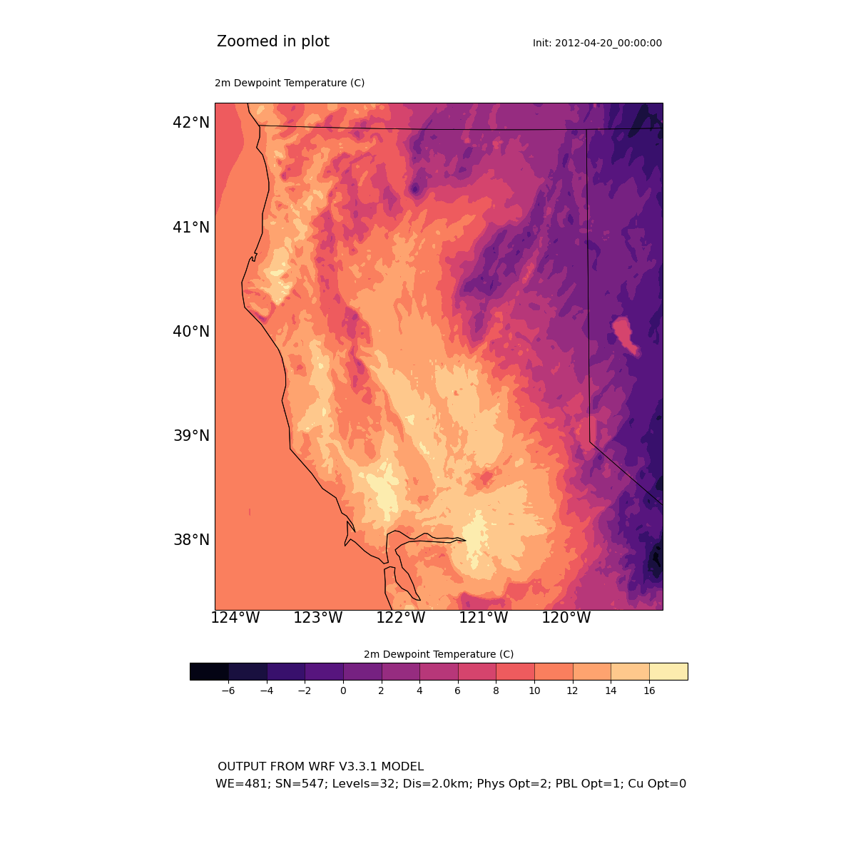
NCL_WRF_zoom_1_2.py

This script illustrates the following concepts:

• Plotting WRF data on native grid

• Subsetting data to ‘zoom in’ on an area

• Plotting data using wrf python functions

• Following best practices when choosing a colormap

See following URLs to see the reproduced NCL plot & script:

• Original NCL script: https://www.ncl.ucar.edu/Applications/Scripts/wrf_zoom_1.ncl

• Original NCL plot: https://www.ncl.ucar.edu/Applications/Images/wrf_zoom_1_2_lg.png

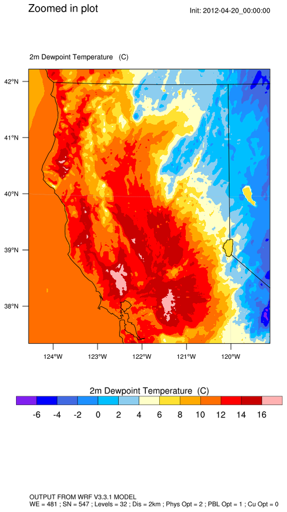
Import packages

from netCDF4 import Dataset
import numpy as np
import matplotlib.pyplot as plt
import matplotlib.ticker as mticker
import cartopy.crs as ccrs
from cartopy.feature import NaturalEarthFeature

from wrf import (getvar, to_np, latlon_coords, get_cartopy)
import geocat.datafiles as gdf

Read in the data

wrfin = Dataset(
    gdf.get("netcdf_files/wrfout_d03_2012-04-22_23_00_00_subset.nc"))
td2 = getvar(wrfin, "td2")

# Set attributes for creating plot titles later
we = getattr(wrfin, 'WEST-EAST_GRID_DIMENSION')
sn = getattr(wrfin, 'SOUTH-NORTH_GRID_DIMENSION')
lvl = getattr(wrfin, 'BOTTOM-TOP_GRID_DIMENSION')
dis = getattr(wrfin, 'DY') / 1000  # Divide by 1000 to go from m to km
phys = getattr(wrfin, 'MP_PHYSICS')
pbl = getattr(wrfin, 'BL_PBL_PHYSICS')
cu = getattr(wrfin, 'CU_PHYSICS')
s_date = getattr(wrfin, 'START_DATE')
str_format = "WE={}; SN={}; Levels={}; Dis={}km; Phys Opt={}; PBL Opt={}; Cu Opt={}"
sd_frmt = "Init: {}"

Create a subset of the data for zoomed in projection

dims = td2.shape

y_start = int(dims[0] / 2)
y_end = int(dims[0] - 1)

x_start = int(0)
x_end = int(dims[1] / 2)

td2_zoom = td2[y_start:y_end, x_start:x_end]

# Define the latitude and longitude coordinates
lats, lons = latlon_coords(td2_zoom)

Plot the data

# The `get_cartopy` wrf function will automatically find and use the
# intended map projection for this dataset
cart_proj = get_cartopy(td2_zoom)

fig = plt.figure(figsize=(12, 12))
ax = plt.axes(projection=cart_proj)

# Add features to the projection
states = NaturalEarthFeature(category="cultural",
                             scale="50m",
                             facecolor="none",
                             name="admin_1_states_provinces")

ax.add_feature(states, linewidth=0.5, edgecolor="black")
ax.coastlines('50m', linewidth=0.8)

# Add filled dew point temperature contours
plt.contourf(to_np(lons),
             to_np(lats),
             to_np(td2_zoom),
             levels=13,
             cmap="magma",
             transform=ccrs.PlateCarree(),
             vmin=-8,
             vmax=18)

# Add a colorbar
cbar = plt.colorbar(ax=ax,
                    orientation="horizontal",
                    ticks=np.arange(-6, 18, 2),
                    drawedges=True,
                    extendrect=True,
                    pad=0.08,
                    shrink=0.75,
                    aspect=30)

# Format location of colorbar text to look like NCL version
cbar.ax.text(0.5,
             1.5,
             '2m Dewpoint Temperature (C)',
             horizontalalignment='center',
             verticalalignment='center',
             transform=cbar.ax.transAxes)

# Format colorbar ticks and labels
cbar.ax.tick_params(labelsize=10)
cbar.ax.get_xaxis().labelpad = -48

# Draw gridlines
gl = ax.gridlines(crs=ccrs.PlateCarree(),
                  draw_labels=True,
                  dms=False,
                  x_inline=False,
                  y_inline=False,
                  linewidth=1,
                  color="k",
                  alpha=0.25)

# Manipulate latitude and longitude gridline numbers and spacing
gl.top_labels = False
gl.right_labels = False
gl.xlocator = mticker.FixedLocator([-120, -121, -122, -123, -124])
gl.ylocator = mticker.FixedLocator([38, 39, 40, 41, 42])
gl.xlabel_style = {"rotation": 0, "size": 15}
gl.ylabel_style = {"rotation": 0, "size": 15}
gl.xlines = False
gl.ylines = False

# Add titles to the plot
plt.title("Zoomed in plot", loc='center', x=.13, y=1.1, size=15)
plt.title("2m Dewpoint Temperature (C)", loc='left', y=1.02, size=10)
plt.title(sd_frmt.format(s_date), loc='right', y=1.1, size=10)

# Add lower text using attributes from the dataset
fig.text(0.25, 0.1, getattr(wrfin, 'TITLE'), size=12)
fig.text(0.252,
         0.08,
         str_format.format(we, sn, lvl, dis, phys, pbl, cu),
         size=12)

plt.show()