fourier_filter_example.py

This script illustrates the following concepts:

• Usage of geocat-comp’s fourier_filter function

• Usage of geocat-datafiles for accessing NetCDF files

See following GitHub repositories to see further information about the function and to access data:

• For fourier_filter function: https://github.com/NCAR/geocat-comp

• For CO-OPS_9415020_wl.csv file: https://github.com/NCAR/geocat-datafiles/tree/main/ascii_files

Dependencies:

• geocat.comp

• geocat.datafiles (Not necessary but for conveniently accessing the data file)

• numpy

• pandas

• xarray

• matplotlib

Import packages

import numpy as np
import pandas as pd
import matplotlib.pyplot as plt
import xarray as xr

import geocat.datafiles as gdf
from geocat.comp import fourier_filter

Read in data:

# Open a netCDF data file using xarray default engine and load the data into xarrays
dataset = xr.DataArray(pd.read_csv(
    gdf.get("ascii_files/CO-OPS_9415020_wl.csv")))
xr_data = dataset.loc[:, 'Verified (ft)']

Plot:

# Set points per hour
data_freq = 10

# Set tide cycle and frequency resolution
tide_freq1 = 1 / (1 * 12.4206)
tide_freq2 = 1 / (2 * 12.4206)
res = data_freq / (len(xr_data))

# Define cutoff_frequency_low and cutoff_frequency_high based on tide frequency
cflow1 = tide_freq1 - res * 5
cfhigh1 = tide_freq1 + res * 5
cflow2 = tide_freq2 - res * 5
cfhigh2 = tide_freq2 + res * 5

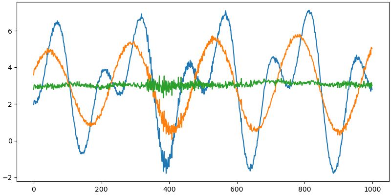
# Generate figure with 1 subplot and set its size (width, height) in inches
fig, ax = plt.subplots(1, 1, dpi=100, figsize=(8, 4), constrained_layout=True)

# Load signal data and plot it
no_tide = xr_data
ax.plot(no_tide[2000:3000])

# Plot filtered signal data using fourier_filter for the first set of cutoffs
no_tide = fourier_filter(no_tide,
                         data_freq,
                         cutoff_frequency_low=cflow1,
                         cutoff_frequency_high=cfhigh1,
                         band_block=True)
ax.plot(no_tide[2000:3000])

# Plot filtered signal data using fourier_filter for the second set of cutoffs
no_tide = fourier_filter(no_tide,
                         data_freq,
                         cutoff_frequency_low=cflow2,
                         cutoff_frequency_high=cfhigh2,
                         band_block=True)
ax.plot(no_tide[2000:3000])

# Show figure
fig.show()

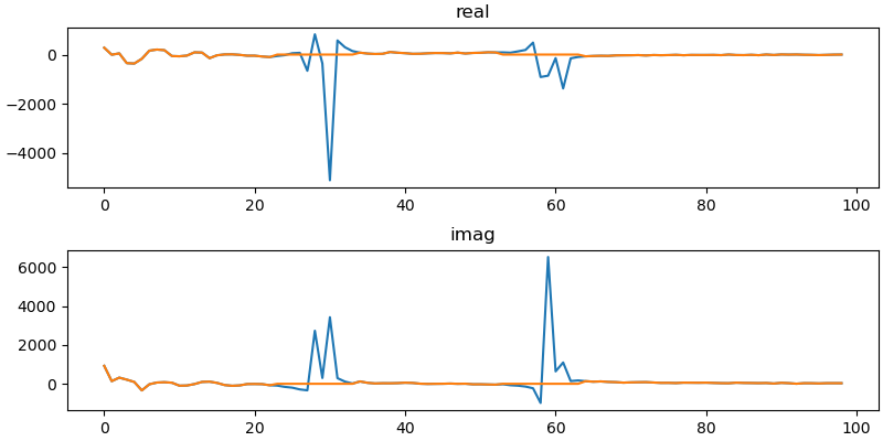
# Generate figure with 2 by 1 subplots and set its size (width, height) in inches
fig, axs = plt.subplots(2, 1, dpi=100, figsize=(8, 4), constrained_layout=True)

# Plot the real set of data utilizing NumPy's Fourier Transform function using both
# the original data and the fourier_filter applied to the second set of cutoffs
axs[0].set_title('real')
axs[0].plot(np.real(np.fft.fft(xr_data)[1:100]))
axs[0].plot(np.real(np.fft.fft(no_tide)[1:100]))

# Plot the imaginary set of data utilizing NumPy's Fourier Transform function using both
# the original data and the fourier_filter applied to the second set of cutoffs
axs[1].set_title('imag')
axs[1].plot(np.imag(np.fft.fft(xr_data)[1:100]))
axs[1].plot(np.imag(np.fft.fft(no_tide)[1:100]))

# Show figure
fig.show()

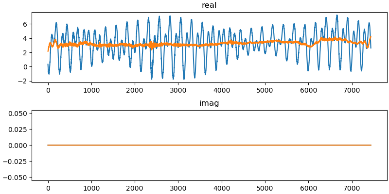
# Generate figure with 2 by 1 subplots and set its size (width, height) in inches
fig, axs = plt.subplots(2, 1, dpi=100, figsize=(8, 4), constrained_layout=True)

# Define start and end of data indices
start = 0
end = -1

# Plot the real and imaginary sets of data from the original and filtered data
axs[0].set_title('real')
axs[0].plot(np.real(xr_data)[start:end])
axs[0].plot(np.real(no_tide)[start:end])
axs[1].set_title('imag')
axs[1].plot(np.imag(xr_data)[start:end])
axs[1].plot(np.imag(no_tide)[start:end])

# Show plot
fig.show()

• 
• 
•