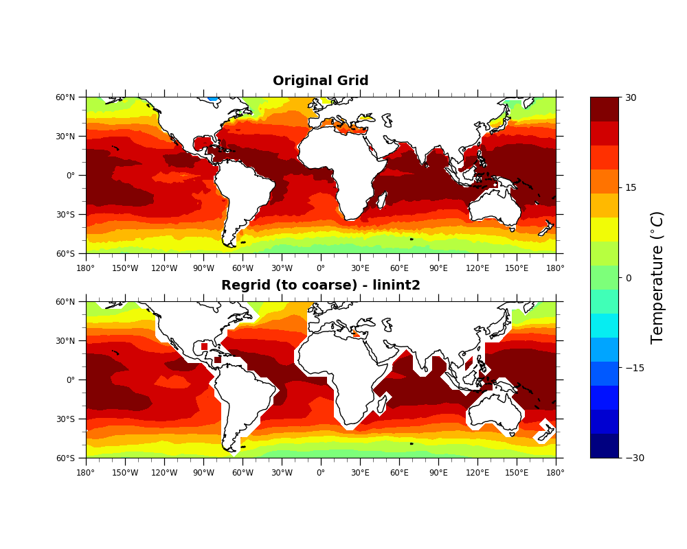
linint2_example.py

This script illustrates the following concepts:

• Usage of geocat-comp’s linint2 function

• Bilinear Interpolation from a rectilinear grid to another rectilinear grid

• Usage of geocat-datafiles for accessing NetCDF files

• Usage of geocat-viz plotting convenience functions

See following GitHub repositories to see further information about the function and to access data:

• For linint2 function: https://github.com/NCAR/geocat-comp

• For “sst.nc” file: https://github.com/NCAR/geocat-datafiles/tree/main/netcdf_files

Dependencies:

• geocat.comp

• geocat.datafiles (Not necessary but for conveniently accessing the NetCDF data file)

• geocat.viz (Not necessary but for plotting convenience)

• numpy

• xarray

• cartopy

• matplotlib

• mpl_toolkits

Import packages:

import cartopy.crs as ccrs
import matplotlib.pyplot as plt
import numpy as np
import xarray as xr
from cartopy.mpl.geoaxes import GeoAxes
from matplotlib import cm
from mpl_toolkits.axes_grid1 import AxesGrid

import geocat.datafiles as gdf
import geocat.viz.util as gvutil
from geocat.comp import linint2

Read in data:

# Open a netCDF data file using xarray default engine and load the data
# into xarray.DataArrays
ds = xr.open_dataset(gdf.get('netcdf_files/sst.nc'))
sst = ds.TEMP[0, 0, :, :].chunk()
lat = ds.LAT[:]
lon = ds.LON[:]

GeoCAT-comp function call:

# Provide (output) interpolation grid
newlat = np.linspace(min(lat), max(lat), 24)
newlon = np.linspace(min(lon), max(lon), 72)

# Invoke `linint2` from `geocat.comp`
newsst = linint2(sst, newlon, newlat, icycx=False)

Plot:

# Generate figure and set its size (width, height) in inches
fig = plt.figure(figsize=(10, 8))

# Generate Axes grid using a Cartopy projection
projection = ccrs.PlateCarree()
axes_class = (GeoAxes, dict(map_projection=projection))
axgr = AxesGrid(fig,
                111,
                axes_class=axes_class,
                nrows_ncols=(2, 1),
                axes_pad=0.7,
                cbar_location='right',
                cbar_mode='single',
                cbar_pad=0.5,
                cbar_size='3%',
                label_mode='')  # note the empty label_mode

# Create a dictionary for common plotting options for both subplots
plot_options = dict(transform=projection,
                    cmap=cm.jet,
                    vmin=-30,
                    vmax=30,
                    levels=16,
                    extend='neither',
                    add_colorbar=False,
                    add_labels=False)

# Plot original grid and linint2 interpolations as two subplots
# within the figure
for i, ax in enumerate(axgr):

    # Plot contours for both the subplots
    if (i == 0):
        sst.plot.contourf(ax=ax, **plot_options)
        ax.set_title('Original Grid', fontsize=14, fontweight='bold', y=1.04)
    else:
        p = newsst.plot.contourf(ax=ax, **plot_options)
        ax.set_title('Regrid (to coarse) - linint2',
                     fontsize=14,
                     fontweight='bold',
                     y=1.04)

    # Add coastlines to the subplots
    ax.coastlines()

    # Use geocat.viz.util convenience function to add minor and major tick
    # lines
    gvutil.add_major_minor_ticks(ax)

    # Use geocat.viz.util convenience function to set axes limits & tick
    # values without calling several matplotlib functions
    gvutil.set_axes_limits_and_ticks(ax,
                                     xticks=np.linspace(-180, 180, 13),
                                     yticks=np.linspace(-60, 60, 5))

    # Use geocat.viz.util convenience function to make plots look like NCL
    # plots by using latitude, longitude tick labels
    gvutil.add_lat_lon_ticklabels(ax, zero_direction_label=False)

# Add color bar and label details (title, size, etc.)
cax = axgr.cbar_axes[0]
cax.colorbar(p)
axis = cax.axis[cax.orientation]
axis.label.set_text(r'Temperature ($^{\circ} C$)')
axis.label.set_size(16)
axis.major_ticklabels.set_size(10)

plt.show()