climatology_average_example.py

This script illustrates the following concepts:

• Usage of geocat-comp’s climatology_average function

• Usage of geocat-datafiles for accessing NetCDF files

• Creating a figure with stacked subplots

See following GitHub repositories to see further information about the function and how to access data:

• For GeoCAT functions: https://github.com/NCAR/geocat-comp

• For atm.20C.hourly6-1990-1995.nc file: https://github.com/NCAR/geocat-datafiles/tree/main/netcdf_files

Dependencies:

• geocat.comp

• geocat.datafiles (for accessing data file only)

• geocat.viz

• cftime (installed with geocat.comp)

• matplotlib (installed with geocat.viz)

• xarray (installed with geocat.comp)

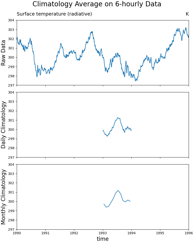
Figure Description: The top subplot is raw surface temperature data from a model run with a temporal resolution of 6-hours.

The middle subplot shows the output of the raw data being aggregated using the climatology_average function with the freq argument set to ‘daily’. This function with that setting finds the average daily temperature for each day of the year. The output has adjusted datetimes instead of using integers to denote the day of the year for the time axis. The year for the outputted data is the floor of the median year of the inputted data, which is 1993 in this case.

The bottom subplot shows the output of climatology_average with the freq argument set to monthly. This works much the same as for the middle plot; however, the data is now grouped by month which yeilds a smoother curve. The time axis is adjusted in the same way, except now there are only 12 data points with one for each month.

Import packages

import cftime
import matplotlib.pyplot as plt
import xarray as xr

from geocat.comp import climatology_average
import geocat.datafiles as gdf
from geocat.viz import util as gvutil

Read in data:

ds = xr.open_dataset(gdf.get('netcdf_files/atm.20C.hourly6-1990-1995-TS.nc'))
ds = ds.isel(member_id=0)  # select one model from the ensemble

temp = ds.TS  # surface temperature data

Calculate daily and monthly climate averages using climatology_average

daily = climatology_average(temp, 'day')
monthly = climatology_average(temp, 'month')

# Convert datetimes to number of hours since 1990-01-01 00:00:00
# This must be done in order to use the time for the x axis
time_num_raw = cftime.date2num(temp.time, 'hours since 1990-01-01 00:00:00')
time_num_day = cftime.date2num(daily.time, 'hours since 1990-01-01 00:00:00')
time_num_month = cftime.date2num(monthly.time,
                                 'hours since 1990-01-01 00:00:00')

# Start and end time for axes limit in units of hours since 1990-01-01 00:00:00
tstart = time_num_raw[0]
tend = time_num_raw[-1]

Plot:

# Make three subplots with shared axes
fig, ax = plt.subplots(3,
                       1,
                       figsize=(8, 10),
                       sharex=True,
                       sharey=True,
                       constrained_layout=True)

# Plot data
ax[0].plot(time_num_raw, temp.data)
ax[1].plot(time_num_day, daily.data)
ax[2].plot(time_num_month, monthly.data)

# Use geocat.viz.util convenience function to set axes parameters without
# calling several matplotlib functions
gvutil.set_axes_limits_and_ticks(ax[0],
                                 xlim=(tstart, tend + 1),
                                 xticks=range(tstart, tend + 1, 365 * 24),
                                 xticklabels=range(1990, 1997),
                                 ylim=(297, 304))

# Use geocat.viz.util convenience function to set titles and labels
gvutil.set_titles_and_labels(ax[0],
                             ylabel='Raw Data',
                             lefttitle=temp.long_name,
                             lefttitlefontsize=14,
                             righttitle=temp.units,
                             righttitlefontsize=14)

gvutil.set_titles_and_labels(ax[1], ylabel='Daily Climatology')

gvutil.set_titles_and_labels(ax[2],
                             ylabel='Monthly Climatology',
                             xlabel=temp.time.long_name)

# Add title manually to control spacing
fig.suptitle('Climatology Average on 6-hourly Data', fontsize=20)

plt.show()