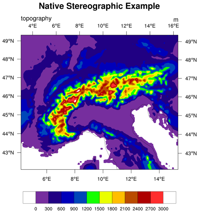
NCL_native_1.py

This script illustrates the following concepts:

• Drawing filled contours over a stereographic map

• Reading in data from binary files

• Setting the view of a stereographic map

• Turning on map tickmark labels with degree symbols

• Choosing colors from a pre-existing colormap

• Making the ends of the colormap white

• Using best practices when choosing plot color scheme to accomodate visual impairments

See following URLs to see the reproduced NCL plot & script:

• Original NCL script: https://www.ncl.ucar.edu/Applications/Scripts/native_1.ncl

• Original NCL plot: https://www.ncl.ucar.edu/Applications/Images/native_1_lg.png

Import packages:

import numpy as np
import cartopy.crs as ccrs
import matplotlib.pyplot as plt
import matplotlib.ticker as mticker

from geocat.viz import util as gvutil
from geocat.viz import cmaps as gvcmaps
import geocat.datafiles as gdf

Read in data:

nlat = 293
nlon = 343

# Read in binary topography file using big endian float data type (>f)
topo = np.fromfile(gdf.get("binary_files/topo.bin"), dtype=np.dtype('>f'))
# Reshape topography array into 2-D array
topo = np.reshape(topo, (nlat, nlon))

# Read in binary latitude/longitude file using big endian float data type (>f)
latlon = np.fromfile(gdf.get("binary_files/latlon.bin"), dtype=np.dtype('>f'))
latlon = np.reshape(latlon, (2, nlat, nlon))
lat = latlon[0]
lon = latlon[1]

Plot:

# Generate figure (set its size (width, height) in inches)
fig = plt.figure(figsize=(10, 10))

# Create cartopy axes and add coastlines
ax = plt.axes(projection=ccrs.NorthPolarStereo(central_longitude=10))
ax.coastlines(linewidths=0.5)

# Set extent to show particular area of the map ranging from 4.25E to 15.25E
# and 42.25N to 49.25N
ax.set_extent([4.25, 15.25, 42.25, 49.25], ccrs.PlateCarree())

# Draw gridlines
gl = ax.gridlines(crs=ccrs.PlateCarree(),
                  draw_labels=True,
                  dms=False,
                  x_inline=False,
                  y_inline=False,
                  linewidth=1,
                  color="black",
                  alpha=0.25)

# Manipulate latitude and longitude gridline numbers and spacing
gl.xlocator = mticker.FixedLocator(np.arange(4, 18, 2))
gl.ylocator = mticker.FixedLocator(np.arange(43, 50))
gl.xlabel_style = {"rotation": 0, "size": 14}
gl.ylabel_style = {"rotation": 0, "size": 14}

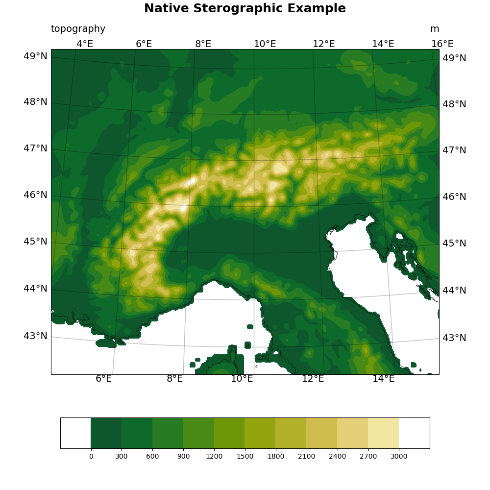
# Create colormap by choosing colors from existing colormap
# The brightness of the colors in cmocean_speed increase linearly. This
# makes the colormap easier to interpret for those with vision impairments
cmap = gvcmaps.cmocean_speed

# Specify the indices of the desired colors
index = [0, 200, 180, 160, 140, 120, 100, 80, 60, 40, 20, 0]
color_list = [cmap[i].colors for i in index]

# make the starting color and end color white
color_list[0] = [1, 1, 1]  # [red, green, blue] values range from 0 to 1
color_list[-1] = [1, 1, 1]

# Plot contour data, use the transform keyword to specify that the data is
# stored as rectangular lon,lat coordinates
contour = ax.contourf(lon,
                      lat,
                      topo,
                      transform=ccrs.PlateCarree(),
                      levels=np.arange(-300, 3301, 300),
                      extend='neither',
                      colors=color_list)

# Create colorbar
plt.colorbar(contour,
             ax=ax,
             ticks=np.arange(0, 3001, 300),
             orientation='horizontal',
             aspect=12,
             pad=0.1,
             shrink=0.8)

# Use geocat.viz.util function to easily set left and right titles
gvutil.set_titles_and_labels(ax,
                             lefttitle="topography",
                             lefttitlefontsize=14,
                             righttitle="m",
                             righttitlefontsize=14)

# Add a main title above the left and right titles
plt.title("Native Sterographic Example",
          loc="center",
          y=1.1,
          size=18,
          fontweight="bold")

# Remove whitespace around plot
plt.tight_layout()

# Show the plot
plt.show()